This post provides an in-depth understanding of Convolutional Neural Networks (CNNs), detailed insights into bedrock operations that power CNNs and step-by-step implementation using PyTorch.

Introduction:

Convolutional Neural Networks (CNNs) are a type of Deep Neural Network (DNN) that are predominantly used in Computer Vision tasks because of their ability to process and analyze visual data, making them significant for a variety of tasks, such as image recognition, object detection, denoising, superresolution and more. CNNs try to work like human visual systems by applying filters to the input data to detect and recognize patterns, making them highly effective in tasks that involve understanding and interpreting images or video data. Typical CNN architecture consists of the following types of layers:

1. Input Layer
2. Convolutional Layer
3. Activation Layer
4. Pooling Layer
5. Fully connected layer
6. Output Layer

1. Input Layer:

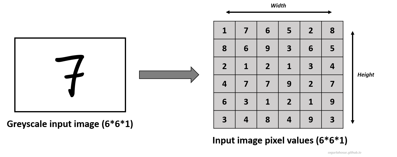
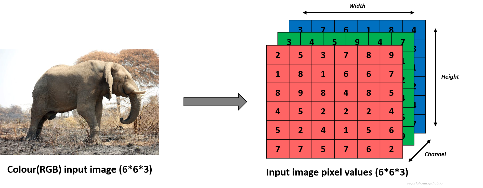
The input layer represents the raw input data, typically a batch of images. Each image is generally represented as a grid of pixels with a single channel if it is a grey image or multiple color channels (red, green, and blue) if it is a color image. This input data is typically called a 3D tensor with three dimensions (height, width, and channels): height and width represent the spatial dimensions of the input data, and channels represent the number of channels. The input layer receives these image data and passes them to the subsequent layers for further processing.

2. Convolutional Layer:

The convolutional layer, often called the Conv Layer, is the building block of Convolutional Neural Networks (CNNs). In this layer, the convolution operation is applied to the data received from the input layer using learnable filters (kernels) to detect local patterns and features available in the input data.

The filter is a small 3D tensor with dimensions (height, width, and channel) that plays a vital role in processing and learning spatial hierarchies of features from input data by sliding over the input feature map in both the height and width dimensions. At each position, the filter performs element-wise multiplication with the portion of the input data it covers, and the results of the element-wise multiplication are summed up to produce a single value. This value is called a feature map value and is placed in the feature map matrix at its respective position.

In the Convolutional layer, each filter is associated with an additional learnable parameter called bias. It is a constant value added to the convolution operation’s output feature map at each spatial position. The bias helps the model to learn better by enabling the activation functions even when the input is zero or when all the inputs to a neuron are zero by allowing shifts in the feature map. It also helps the model account for systematic errors or biases in the data or the network’s predictions.

In mathematical terms, if $\mathbf{W}$ represents the weights of the filter and $\mathbf{b}$ represents the bias term, the output of a convolution operation $\text{Conv}(\mathbf{I}, \mathbf{W}) $ for an input image $\mathbf{I} $ can be represented as:

The filter’s sliding across the complete input is controlled by parameter stride. If stride=1 means, the filter slides/moves one pixel at a time, and if stride=2, the filter slides two pixels at a time simultaneously. Along with stride, one more parameter called padding is used to control the spatial dimensions of the output feature map. When padding =0, the filter is only moved on positions where the input data is present, and there is no additional padding around the input. After we discuss the convolution operation completely, we shall discuss the stride and padding operations in detail to understand their importance.

i. Single channel input convolution:

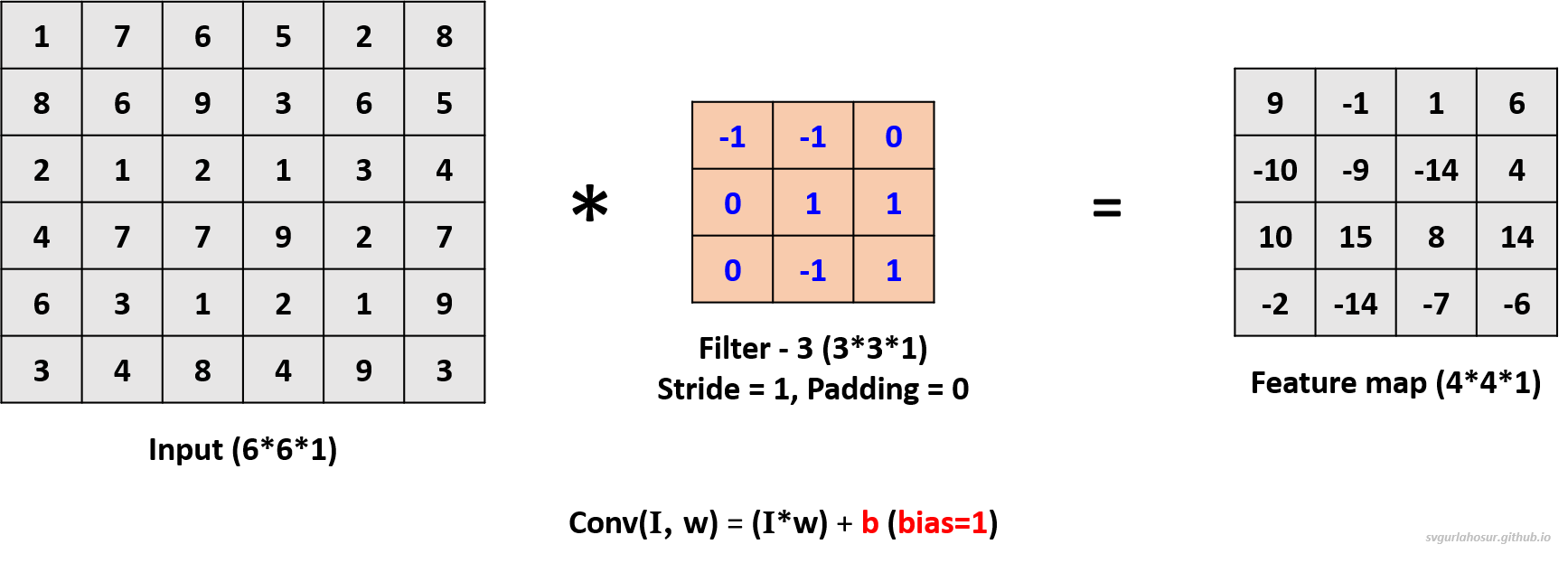
Let us consider the greyscale image data and apply one filter to understand the convolution operation. Since the channel dimension of input data is 1, the kernel will also have a channel dimension of 1, and we shall create a filter with the other two dimensions, height=3 and width=3. We shall consider this filter’s bias value = 2 during the convolution operation to create the feature map.

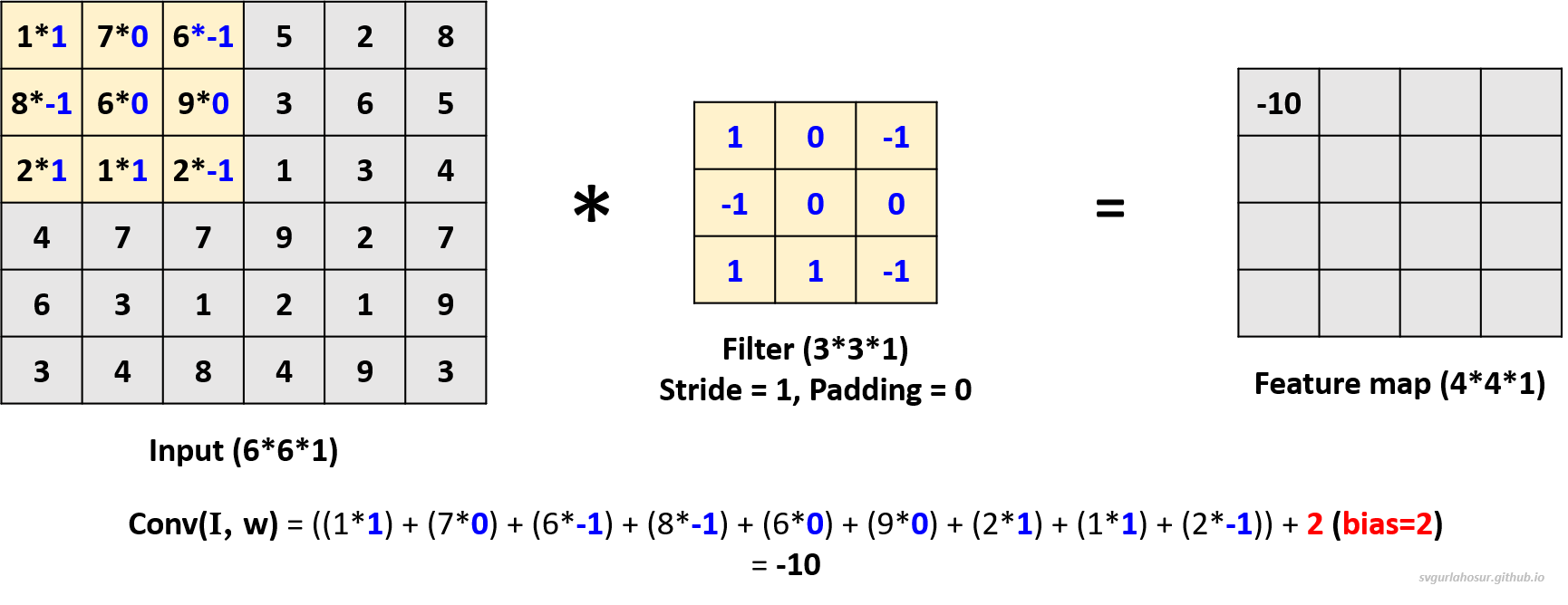
Now, the filter slides one pixel/cell at a time (stride_size=1), calculates the next feature map value, and is placed in the feature map matrix at its respective position. This process will be repeated over the entire input data, and the feature map for the whole input data is calculated.

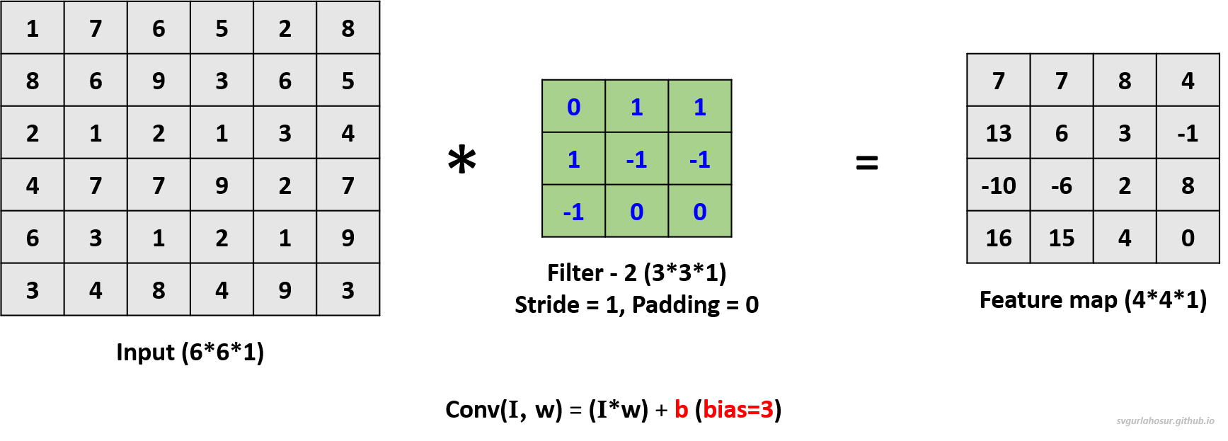
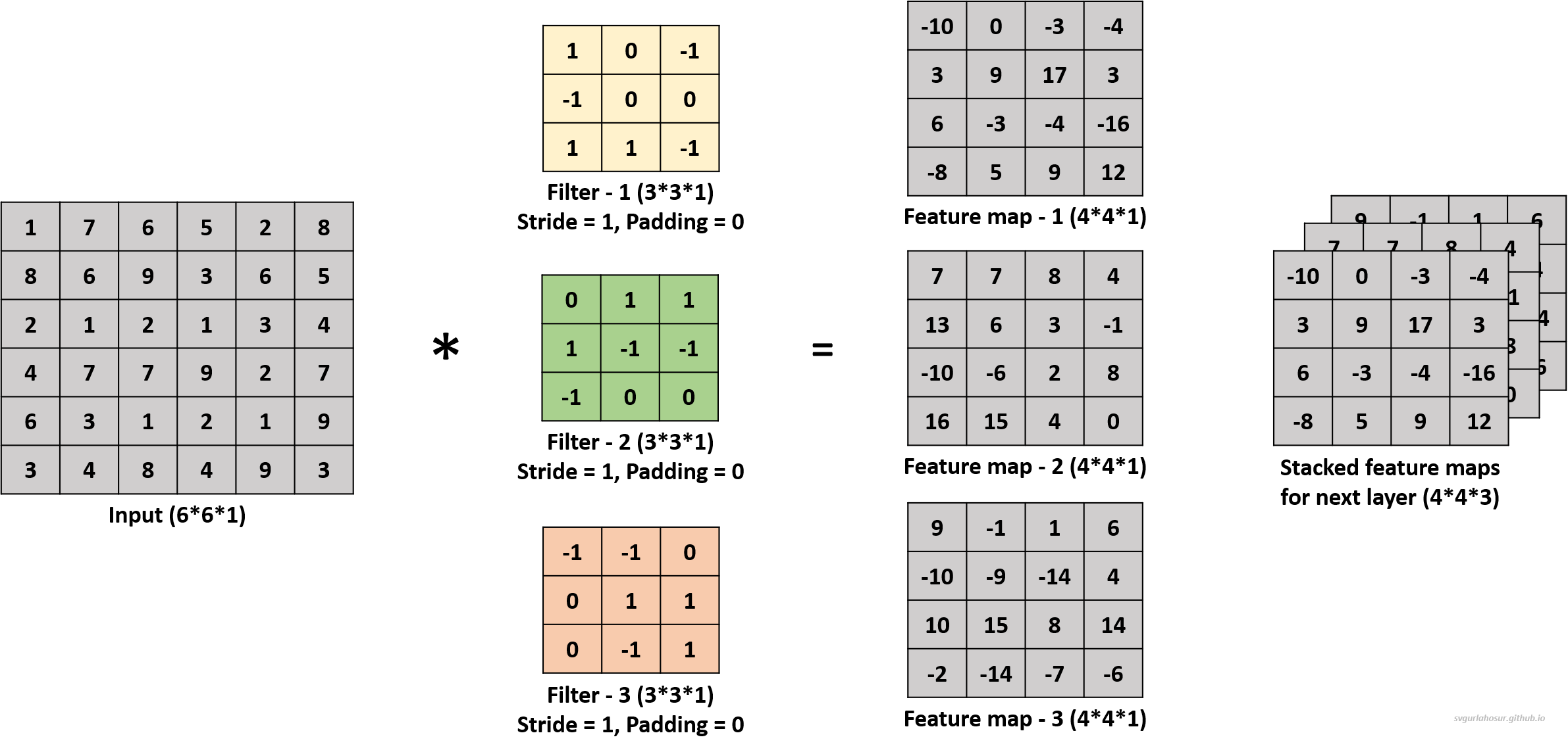
We can use multiple filters on the input image data and calculate the feature maps. The analogy is that the greater the number of filters, the more different feature maps are created that encode information about specific features or patterns in the input data. Hence, let us create two more filters and apply the convolution operation to calculate the feature maps.

For the second filter, let us use the filter’s bias value = 3 during the convolution operation to create the feature map.

For the third filter, let us use the filter’s bias value = 1 during the convolution operation to create the feature map.

We applied a total of three filters, each of dimension \(3*3*1\), to the input data with the dimension \(6*6*1\) and calculated three feature maps of the size \(4*4*3\).

So, the convolution operation uses a filter, a small 3-D tensor containing trainable parameters/weights, which is convolved across the input data by performing element-wise multiplication, summation, and addition of constant bias value, producing a feature map that captures the presence of specific features in the input. Here, the performance of the CNN depends upon the number of feature maps, values present in feature maps, and the shape/size of the feature maps since they contribute to the network’s ability to recognize and classify complex visual data. So, the values in the feature maps depend on the trainable parameters of filters during CNN training, the number of feature maps is dependent on the number of filters used, and the shape of the feature maps is influenced by factors such as input size, filter size, stride, and padding.

The formula for calculating the feature map’s spatial dimensions (height and width) in a convolutional layer, given the input dimensions, kernel size, stride, and padding, can be expressed as follows.

Feature map height: $=(\lfloor\frac{H-F+2P}{S}\rfloor+1)$ and Feature map width: $=(\lfloor\frac{W-F+2P}{S}\rfloor+1)$

• $H$ is the height of the input for convolution operation.
• $W$ is the width of the input for convolution operation.
• $F$ is the height/width (filter is usually square shape) of convolutional filter.
• $P$ is the amount of padding applied to input.
• $S$ is the stride for convolution operation.

Now, let us take a few use cases to understand this.

1. Consider an input of shape \((6*6*1)\), so let us perform the convolution operation with a filter \((4*4*1)\), stride=1, and padding=0.

• Feature map height \(=(\lfloor\frac{H-F+2P}{S}\rfloor+1)\) \(=(\lfloor\frac{6-4+(2*0)}{1}\rfloor+1)\) \(=(\lfloor\frac{2}{1}\rfloor+1)\) \(=3\)
• Feature map width \(=(\lfloor\frac{H-F+2P}{S}\rfloor+1)\) \(=(\lfloor\frac{6-4+(2*0)}{1}\rfloor+1)\) \(=(\lfloor\frac{2}{1}\rfloor+1)\) \(=3\)

2. Consider an input of shape \((6*6*1)\), so let us perform the convolution operation with a filter \((4*4*1)\), stride=2, and padding=0.

• Feature map height \(=(\lfloor\frac{H-F+2P}{S}\rfloor+1)\) \(=(\lfloor\frac{6-4+(2*0)}{2}\rfloor+1)\) \(=(\lfloor\frac{2}{2}\rfloor+1)\) \(=2\)
• Feature map width \(=(\lfloor\frac{H-F+2P}{S}\rfloor+1)\) \(=(\lfloor\frac{6-4+(2*0)}{2}\rfloor+1)\) \(=(\lfloor\frac{2}{2}\rfloor+1)\) \(=2\)

3. Consider an input of shape \((6*6*1)\), so let us perform the convolution operation with a filter \((4*4*1)\), stride=2, and padding=1. For padding = 1, one unit of padding is added to all sides of the input. This padding is typically filled with zeros, ensuring that the convolutional kernel can be applied to all positions in the input, including the border pixels.

• Feature map height \(=(\lfloor\frac{H-F+2P}{S}\rfloor+1)\) \(=(\lfloor\frac{6-4+(2*1)}{2}\rfloor+1)\) \(=(\lfloor\frac{4}{2}\rfloor+1)\) \(=3\)
• Feature map width \(=(\lfloor\frac{H-F+2P}{S}\rfloor+1)\) \(=(\lfloor\frac{6-4+(2*1)}{2}\rfloor+1)\) \(=(\lfloor\frac{4}{2}\rfloor+1)\) \(=3\)

Visit “this post” to learn more about how the feature map size and values are calculated by playing with different input, stride, padding, and kernel size values.

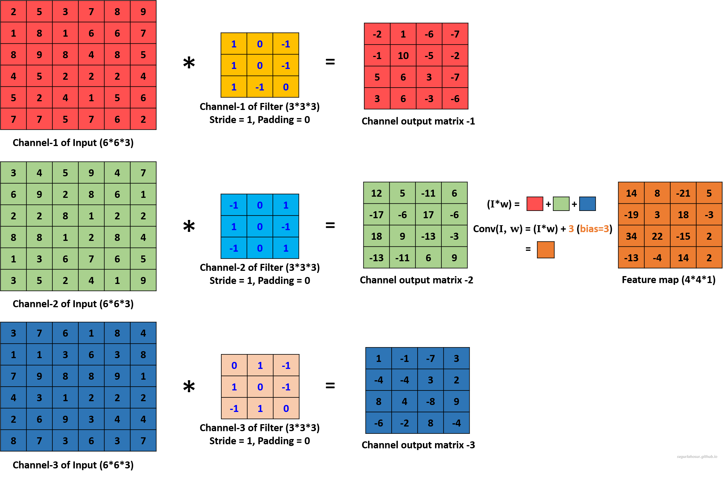
ii. Multi-channel input convolution:

To understand how convolution works for a color image, let us consider the color image data and apply one filter to understand the convolution operation. Now the channel dimension of input data is 3, the kernel/filter will also have a channel dimension of 3, and we shall create a filter with the other two dimensions, height=3 and width=3.

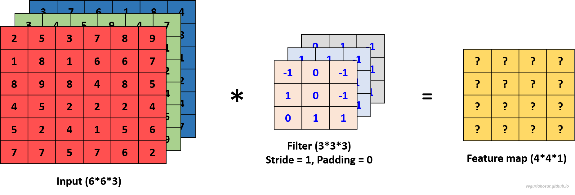
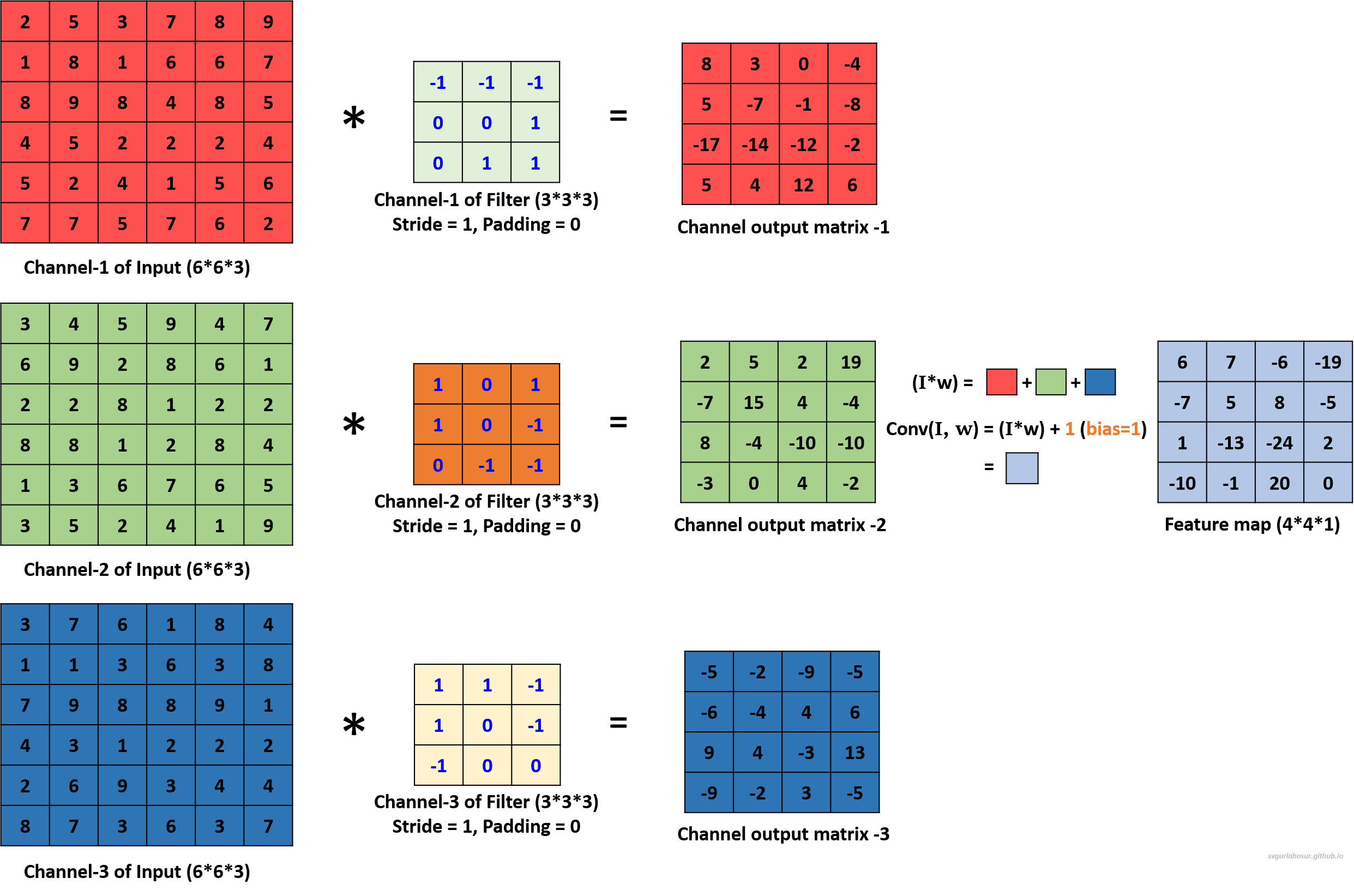
During convolution with multiple-channel input data, a filter is used with the number of channels that are the same as the number of channels in the input data. Each channel of the filter handles one channel of input and performs element-wise multiplication and summation with the portion of the input data it covers. The value is stored in their respective channel output matrix. Once the values are calculated for all the channel output matrices, the element-wise sum is calculated across all the channel output matrices, and a constant bias term is added to the sum before storing the value in the feature map matrix.

In mathematical terms, if $\mathbf{I}$ represents the input tensor with multiple channels, $\mathbf{W}$ denotes the filter tensor, and $\mathbf{b}$ represents the bias term, the convolution operation for multi-channel input can be represented as:

Where:

• $C_{in}$ is the total number of channels in the input tensor.
• $\mathbf{I}_i $ is the $i^{th}$ channel of the input tensor.
• $\mathbf{W}_i $ is the corresponding filter channel for the $i^{th}$ input tensor channel.
• $\mathbf{(*)}$ denotes the convolution operation between a single channel of the input and its corresponding filter.

Now, the filter slides one pixel/cell at a time (stride_size=1) and calculates the channel output matrix values and the feature map matrix. This process will be repeated over the entire input data, and the feature map values for the whole input data are calculated.

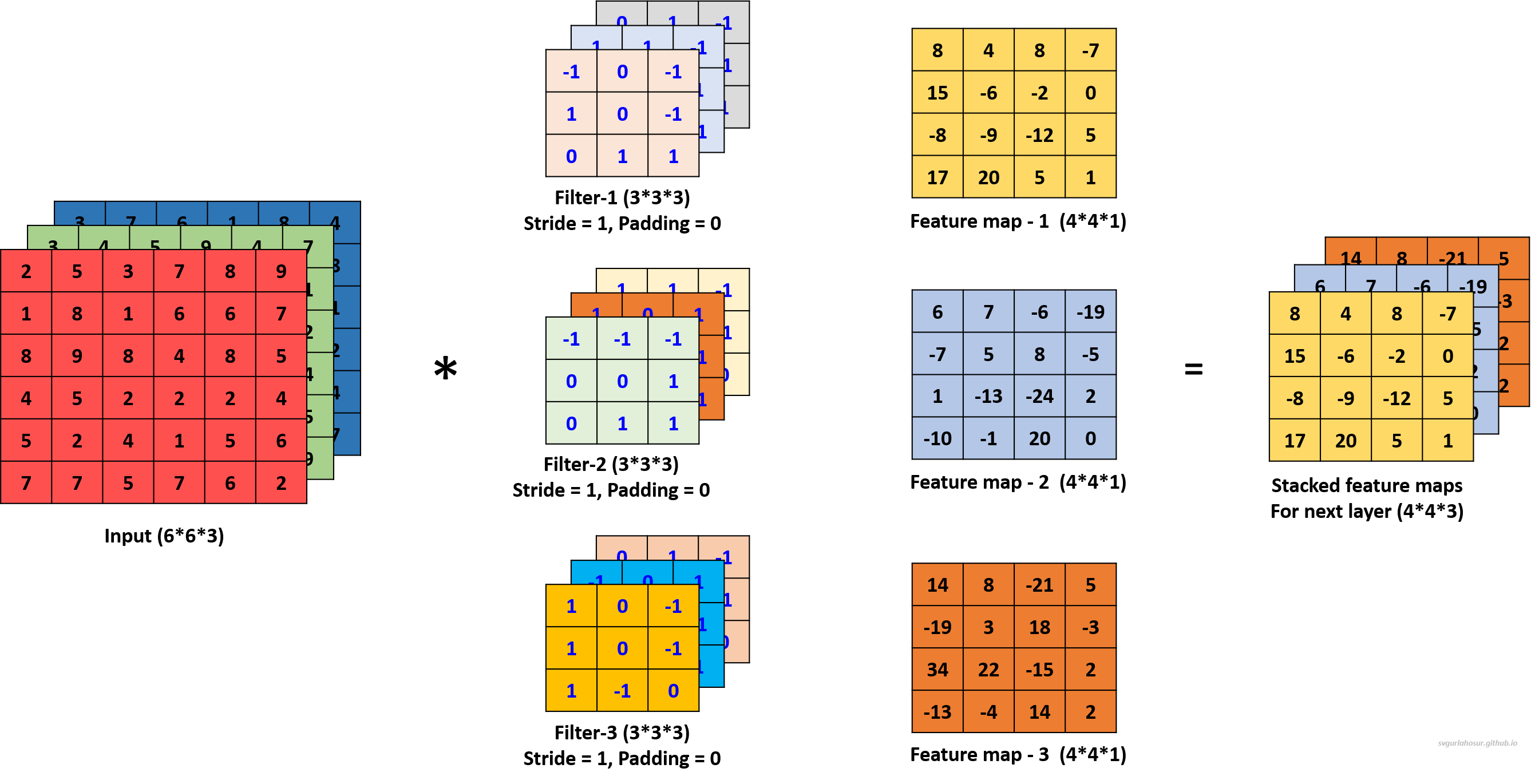
We can use multiple filters on the multi-channel input image data and calculate the feature maps to encode more information about specific features or patterns in the input data. Hence, let us create two more filters and apply the convolution operation to calculate the feature maps.

For the second filter, let us use the filter’s bias value = 1 during the convolution operation to create the feature map.

For the third filter, let us use the filter’s bias value = 3 during the convolution operation to create the feature map.

We applied a total of three filters, each of dimension 3∗3∗3, to the input data with the dimension 6∗6∗3 and calculated three feature maps of the size 4∗4∗3.

3. Activation Layer:

In Machine Learning models, linearity/linear systems refer to the ability to represent the model as a complex function with a linear combination of input features and weights/parameters. Usually, Deep Learning models like CNNs are built to solve non-linear systems/non-linear problems. Hence, if we do not introduce non-linearity into the neural network model, the designed neural network model will be a linear model that cannot capture complex patterns in data. So, the activation layer applies an activation function to feature maps produced from the convolutional layer to bring non-linearity into the network, allowing the network to learn and represent more complex relationships between features present in the input data.

The commonly used activation functions in CNNs are as follows:

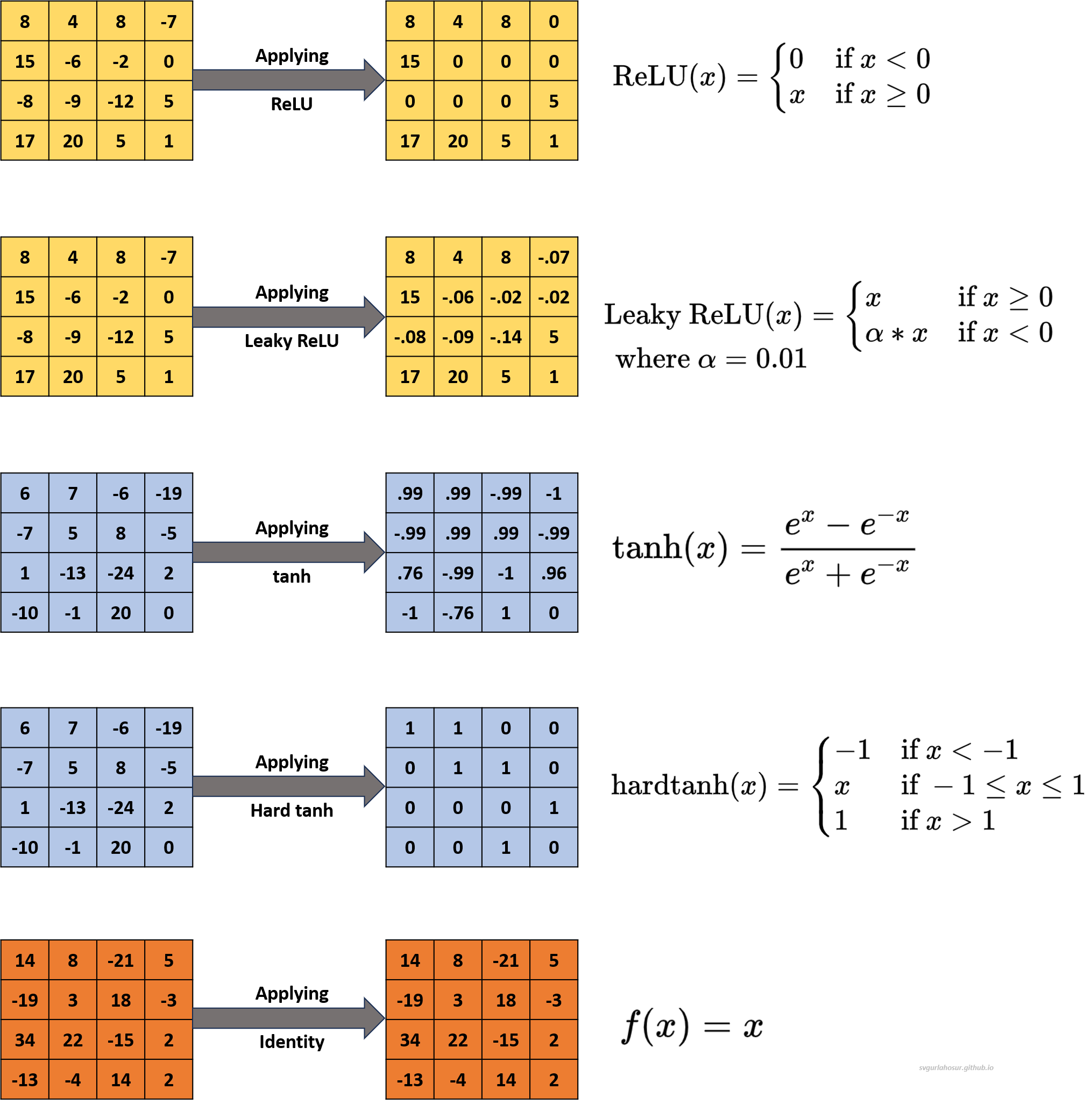
1. Rectified Linear Unit (ReLU): The ReLU is one of the most widely used activation function during the design of CNNs. This function will replace all the negative values in the feature maps produced by the convolution layer with zero and leave positive values unchanged. Because of converting negative values to zeroes, sometimes, the filters in the networks may become inactive/stop while training. The ReLU can be defined as,

2. Leaky ReLU: The Leaky ReLU replaces all the negative values in the feature maps produced by the convolution layer with a small positive constant and leaves positive values unchanged. This function will solve the problem of networks becoming inactive/stop while training by allowing a small, non-zero gradient for negative inputs. The Leaky ReLU can be defined as,

3. Hyperbolic Tangent (tanh): Tanh squashes input values between -1 and 1, making it zero-centered. Tanh is sometimes preferred over sigmoid when the data distribution is centered around zero. Mathematically, it can be defined as,

4. Hard Tanh (Hard Hyperbolic Tangent): The Hard Tanh activation function is a hyperbolic tangent (tanh) function variation. The tanh squashes input values to the range [-1, 1], and the hard tanh clips input values to the range [0, 1]. The goal is to maintain the non-linearity of the tanh function while preventing extreme values. The Hard Tanh function is defined as,

5. Linear Activation (Identity Function): Linear Activation is one of the simplest activation functions used in neural networks. Unlike other activation functions that introduce non-linearities, the identity function does not alter the input and outputs the input value directly. The identity function is defined as, $f(x) = x$.

4. Pooling Layer:

In Convolutional Neural Networks, the pooling Layer downsizes the feature maps from the activation layer while retaining essential information to enable the network to focus on the most critical information in the input data. The pooling operation is usually applied after the convolution layer to gradually decrease the spatial resolution of the feature maps and decrease the number of filters/parameters in the network to prevent overfitting and reduce computational complexity. There are two common types of pooling operations: Max Pooling and Average Pooling.

1. In the max pooling, the maximum value is selected within a specified pooling window from the input feature map. This operation retains the most salient features, discarding less relevant information.

2. In average pooling, the average value is calculated within a specified pooling window from the input feature. Like max pooling, average pooling helps downsample and retain the most salient features from the input feature map but takes the average instead of the maximum.

The formula for calculating the spatial dimensions (height and width) of the output feature map after applying Pooling operation in a Convolutional Neural Network is given by:

Feature map height: $=(\frac{H}{F})$ and Feature map width: $=(\frac{W}{F})$

• $H$ is the height of the input for pooling operation.
• $W$ is the width of the input for pooling operation.
• $F$ is the height/width (window is usually square shape) of pooling window (pool size).

Now, let us take a few use cases to understand this.

1. Consider an input of feature map with shape \((4*4*1)\), so let us perform the max pooling operation with a pooling window \((2*2*1)\).

• Feature map height \(=(\frac{H}{F})\) \(=(\frac{4}{2})\) \(=2\)
• Feature map width \(=(\frac{H}{F})\) \(=(\frac{4}{2})\) \(=2\)

2. Consider an input of feature map with shape \((4*4*1)\), so let us perform the average pooling operation with a pooling window \((2*2*1)\).

• Feature map height \(=(\frac{H}{F})\) \(=(\frac{4}{2})\) \(=2\)
• Feature map width \(=(\frac{H}{F})\) \(=(\frac{4}{2})\) \(=2\)

Visit “this post” to learn more about how the feature map size and values are calculated by playing with different inputs and pooling filter size values.

5. Fully connected layer:

In the fully connected layer (dense layer), the condensed feature maps from the pooling layers are flattened into a 1D vector, serving as the input to the neurons in the fully connected layer. These layers perform traditional feedforward operations, multiplying the input by learnable weights and adding biases, followed by an activation function. Comprising one or more fully connected layers that connect every neuron to the preceding layer, it leverages high-level features learned from earlier convolutional and pooling layers to produce class scores or predictions. The connections are associated with weights learned during the training process through backpropagation and optimization algorithms. These layers are vital for capturing complex relationships within the data, playing a critical role in making final predictions or classifications, thus making them an essential component in designing neural networks for computer vision tasks. The operation performed at each neuron in a fully connected layer can be expressed as follows:

$\text{Output} = \text{Activation}(\text{input} \times \text{weights} + \text{bias})$

• $input$ is the flattened vector from the pooling layer.
• $weights$ are the learnable parameters associated with each connection.
• $bias$ is an additional learnable parameter added to each neuron.
• $Activation$ is an activation function applied to the input recieved at hidden layers to calculate output of neuron. Common activation functions in fully connected layers include ReLU, LeakyReLU, sigmoid, or tanh.

Now, let us consider the feature map from Figure 17 and flatten it to build a fully connected layer with two layers. The first fully connected layer will have four neurons; since the flattened feature map has four tensors. We shall use three neurons in the second, and let us consider this last (second) layer in the fully connected layer as the hidden layer since the last/output layer will be there to receive to the output from hidden layer for producing the final predictions based on the features learned by the network from the input data.

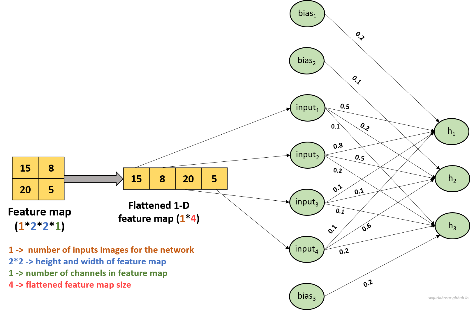
Input feature map matrix:

The flattened 1-D tensor input:

Let us consider the weights and biases for the fully connected layer as follows with ReLU Activation Function.

The weights and bias between inputs and first neuron $(h_1)$ in hidden layer as: $W_1 = [0.5, 0.8, 0.1, 0.1]$, $b_1 = 0.2$.

The weights and bias between inputs and second neuron $(h_2)$ in hidden layer as: $W_2 = [0.2, 0.5, 0.1, 0.6]$, $b_2 = 0.1$.

The weights and bias between inputs and third neuron $(h_3)$ in hidden layer as: $W_3 = [0.1, 0.2, 0.1, 0.2]$, $b_3 = 0.3$.

Now, we shall calculate the output for each neuron in the hidden layer:

So, the output from the the three neurons in the hidden layer (last layer in the fully conncted layer) are as follows:

6. Output Layer:

The output layer is the final layer responsible for producing the network’s predictions. Its design varies depending on the specific task. In image classification, the output layer typically consists of neurons corresponding to different classes, and a softmax/log-softmax activation function is applied to convert the neuron’s raw scores into class probabilities, allowing the network to predict the most likely class. The output layer may have a different object detection or image segmentation structure, providing detailed information about object locations or pixel-wise segmentations. The output layer effectively transforms the high-level features extracted by the network into the desired output format, making it a critical component that determines the network’s function.

Now, let us consider that the output layer has to perform image classification, and three types of classes/labels (Lion, Tiger and Elephant) are present in the input data. Then, we need three neurons in the output layer to represent the three classes. These three neurons will be connected to all neurons in the last layer of the fully connected layer($h_1, h_2, h_3$) with the help of weights and bias to produce the output.

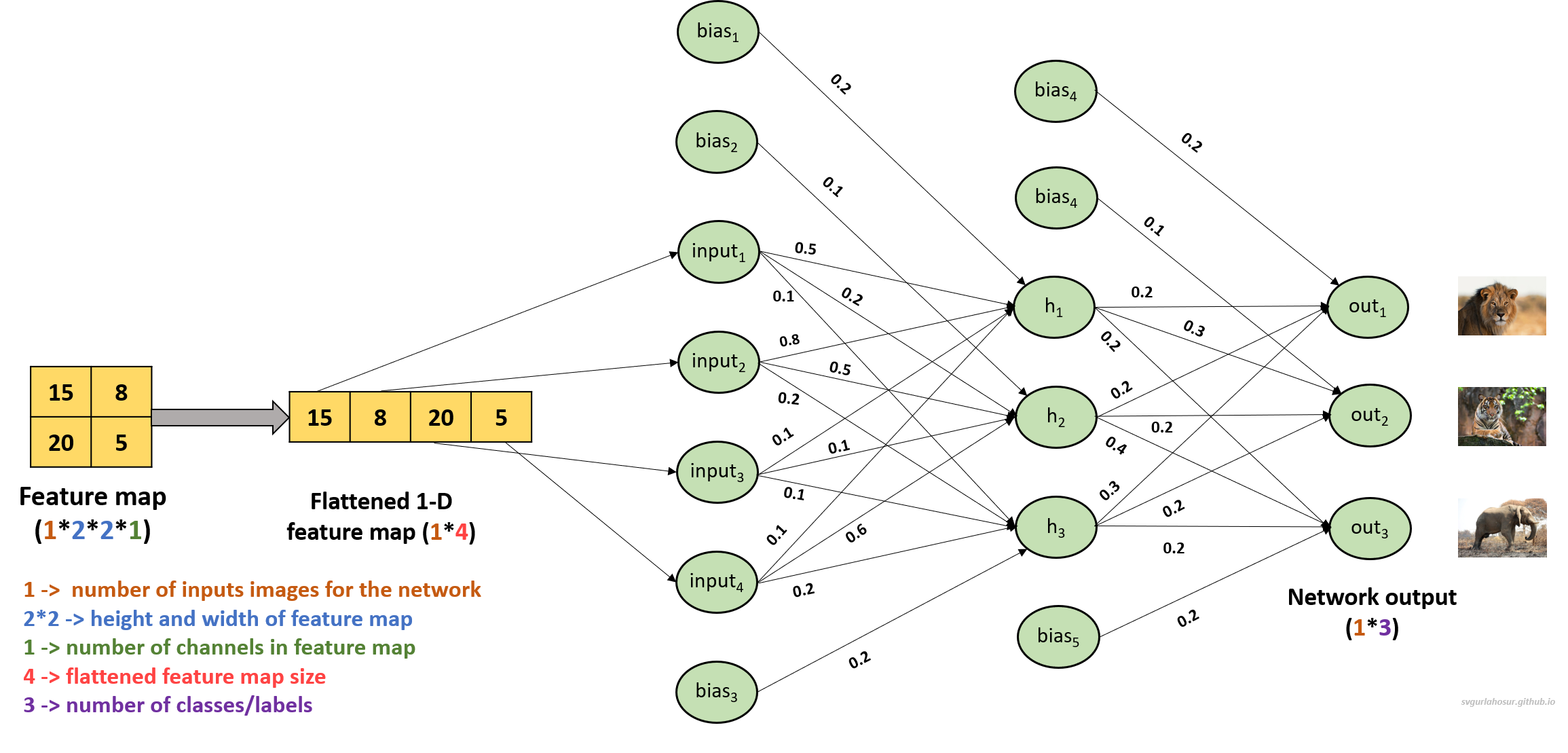
Let us calculate the output from the output layer neurons ($out_1, out_2, out_3$) and see the prediction from the network with weights and bias as follows.

The weights and bias between hidden layer outputs and first neuron $(out_1)$ in output layer as: $W_4 = [0.2, 0.2, 0.3]$, $b_4 = 0.2$.

The weights and bias between hidden layer outputs and second neuron $(out_2)$ in output layer as: $W_5 = [0.3, 0.2, 0.2]$, $b_5 = 0.1$.

The weights and bias between hidden layer outputs and third neuron $(out_3)$ in output layer as: $W_6 = [0.2, 0.4, 0.2]$, $b_6 = 0.2$.

The output received at each output layer neuron is as follows:

Let us consider $[0, 0, 1]$, the expected output from the network, with the assumption that given input belongs to the class elephant. We shall apply CrossEntropy Loss, which is commonly used in classification problems with multiple classes, to calculate the output probabilities and the loss(error) from the network.

Cross Entropy Loss measures the performance of a classification model whose output is a probability value between 0 and 1. The mathematical formula for CrossEntropy loss between predicted and target values can be expressed as:

Where:

• $N$ is the number of classes or outputs.
• $y_{i}$ represents the target value for the $i^th$ class.
• $\hat{out}_{i}$ represents the predicted probability for the $i^th$ class.

We have three neurons in the output layer (three classes), and the predicted values are 7.86, 8.78, and 9.64. Since these values do not represent probabilities (values should be between 0 and 1), we shall apply the softmax function to transform them into probabilities before calculating the loss.

Where:

• $\text{logits}$ are the unnormalized predictions.
• $C$ is the number of classes.

Now, applying the CrossEntropy loss formula:

So, for the network to predict the correct class of the given input image of the elephant as an elephant, the Cross-Entropy Loss is 0.464866 at the output neuron $out_3$. This Cross-Entropy Loss at the output layer will be used for network optimization in backpropagation so that in the subsequent forward propagation, the loss will be less compared to the previous loss. In reality, multiple images will be sent to the network instead of one single image to calculate the predictions and cross-entropy loss. Then, the model parameters will be updated to efficiently classify the given inputs to their correct class with the least error.

The process of defining the CNN architecture, sending input data, predicting output, calculating loss, and adjusting model parameters to minimize the loss is called model training. The number of images that are sent to the model for training is defined by the hyperparameter batch_size, and the specific number for batch_size depends upon the design choice, resource availability, model, and dataset complexity.

Let us take one more example where we shall take three images as input (batch_size=3) and calculate the total error from the network calculated.

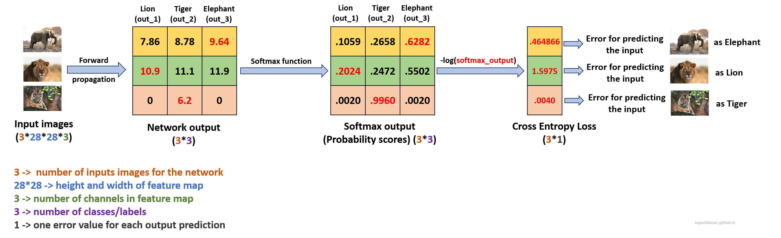
The total Cross Entropy Loss for network with all the three images = (.464866 + 1.5975 + .0040)/3 = 0.688788. For Elephant image, the error is not very large since probability score is moderate for its respective output neuron (out_3). For the Lion image, the error is large since probability score is less for its respective output neuron (out_1). For Tiger image, the error is less since probability score is large for its respective output neuron (out_2).

With an optimal batch size, model training is carried out where input data convolves through filters, passes through activation functions, and undergoes pooling to extract relevant features. The final layer produces predictions, which are compared against the target labels using the Cross-Entropy Loss function. This loss quantifies the dissimilarity between predicted and actual values, measuring the network’s performance. The Cross-Entropy Loss at the output layer will be used for network optimization in backpropagation so that in the subsequent forward propagation, the loss will be less compared to the previous loss.

In the backpropagation phase, gradients of this cross-entropy loss with respect to every network parameter are computed. It involves differentiating the loss function with regard to weights, biases, and filter values. These gradients signify how much a change in each parameter would affect the overall loss. Utilizing these gradients, optimization algorithms like stochastic gradient descent update the parameters. Weights and biases in fully connected layers and the kernels in convolutional layers are adjusted incrementally in the opposite direction of the gradients to minimize the loss. At each iteration (one forward and one backward propagation), all the network’s parameters are refined, enabling it to learn more complex patterns in the data.

This iterative process of forward propagation, loss calculation, backpropagation, and parameter updation slowly optimizes the CNN to recognize complex patterns in the data, yielding improved performance and more accurate predictions.

So, in the “next post”, we do a from-scratch implementation of the Convolutional Neural Network using PyTorch for image classification tasks using the CIFAR-10 dataset. We shall practically see how the convolutional neural network takes images as input, produces output, and minimizes errors to improve the model performance of the image classification task.

7. References

1. Machine Learning, Tom Mitchell, McGraw Hill, 1997.
2. “CS229: Machine Learning” course by Andrew N G at Stanford, Autumn 2018.