
Mastering Multilayer Perceptrons: understanding forward and backpropagation with numerical example using Python.
Published:
This post discusses Neural Networks, particularly Multilayer Perceptron (MLP), and delves with a step-by-step numerical example for forward and backpropagation along with its Python implementation.
Introduction
The Multi-layer Perceptron is a powerful and popular neural network architecture that has significantly impacted machine learning, pattern recognition, and deep learning. MLPs are known for learning intricate patterns and making precise predictions. This post focuses on the detailed analysis of forward and backpropagation in MLPs, examining their fundamental concepts, mechanisms, advantages, difficulties, and influence on artificial intelligence.
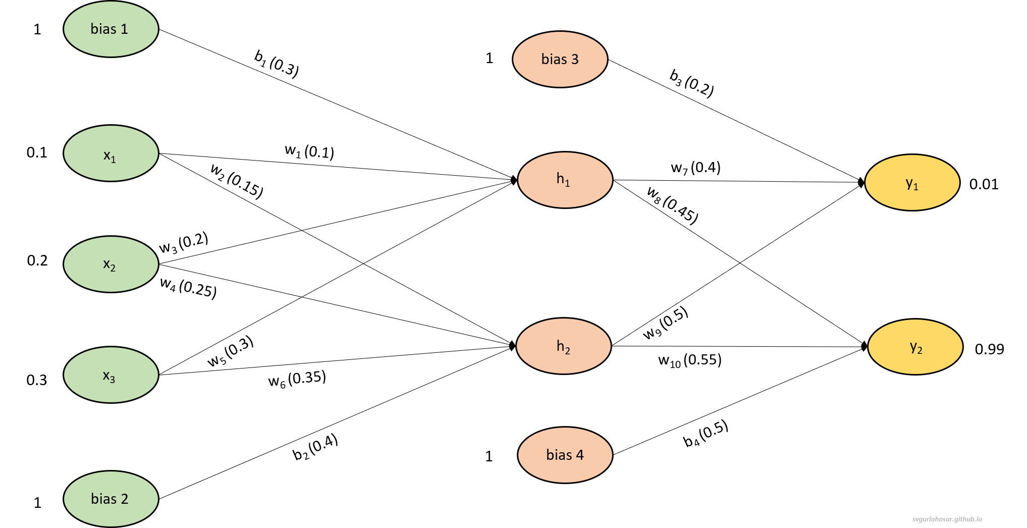
The structure/design of every MLP will have one input layer, one or more hidden layers, and one output layer. The MLP shown in Figure 1 has one input layer, one hidden layer, and one output layer. The input layer has three input neurons represented by the three nodes ($x_1, x_2, x_3$) in the input layer and two bias neurons represented by the two bias nodes ($b_1, b_2$). The hidden layer consists of two neurons, also known as hidden units ($h_1, h_2$) and two bias units ($b_3, b_4$). The output layer has a total of two neurons ($y_1, y_2$). The number of neurons in the input layer is determined by the number of features/inputs. If the input is an image, then the total number of pixels. The number of layers and number of neurons in each hidden layer is determined by the problem being solved and the AI designer. The number of neurons in the output layer depends on the problem being solved. For example, two output neurons might represent the two possible classes in a binary classification task.
The training of MLP mainly involves two steps: forward propagation and backpropagation. Forward propagation refers to calculating the output of an MLP for a given set of input data. Backpropagation is used to update the weights and biases of the neural network to minimize the error or loss function based on the gradients so that the predicted output will be same or as close as possible to the actual output.
Note:
There is sometimes a debate over whether we should update the biases in backpropagation along with weights during MLP training or not. Updating both in an MLP is essential since biases enable the introduction of non-linearity through activation functions, preventing vanishing and exploding gradients and ensuring stable training. Biases also break the symmetry during initialization, making MLP generalize and adapt to various data distributions.
Hence, in this post, both variations are covered, and analysis from the point of loss is carried out to justify that the updation of biases leads to better network convergence during gradient descent optimization.
1. Forward propagation
The Forward propagation, also known as feedforward, is the initial phase of training an MLP. It involves passing input data through the network’s layers, where each neuron calculates a weighted sum of its inputs and applies an activation function to produce an output. The process continues layer by layer until the final layer generates the network’s prediction. This process can divided into the following steps:
- Initialization of inputs and network parameters: The input layer is initialized with the input data, and all the neurons and biases of MLP will be initialized with some initial values.
- Weighted Sum Calculation: Each neuron in the current layer computes the weighted sum of its inputs, including the inputs, corresponding weights, and biases.
- Activation Function: The weighted sum is then passed through an activation function, introducing non-linearity into the network. The specific type of activation function used can vary, but common choices include the sigmoid, tanh, or relu functions. In this discussion, we have considered the sigmoid as the activation function.
- Intermediate Output calculation: The outputs from the current layer are sent as inputs to the next layer.
- Iteration: Steps 2-4 are repeated for all the hidden layers until the output layer is reached.
- Network output calculation: The final layer’s output values act as the network’s prediction and are used to improve the network performance further by calculating the error by comparing them against the actual outputs for the network.
Overall, the MLP in Figure 1 with the mentioned initial values for weights and bias performs forward propagation by passing the input data through the hidden layer to the output layer, with each neuron applying weights and activation functions and producing outputs. In the considered example, with the current inputs ($x_1, x_2, x_3$), the network has to predict the outputs using all weights ($w_1, w_2, w_3, w_4, w_5, w_6, w_7, w_8, w_9 ,w_{10}$) and biases ($b_1, b_2, b_3, b_4$) so that the predicted output from node $y_1$ to be 0.01 and node $y_2$ to be 0.99.
i. Input and output at hidden layer:
First, let us calculate the input and output at the hidden layer neurons $h_1$ and $h_2$ with the given three inputs $x_1$, $x_2$, $x_3$ and two biases $b_1$, $b_2$.
\[in_{h1}=w_1 * x_1+w_3 * x_2+w_5 * x_3+b_1 * 1\] \[in_{h1}=0.1 * 0.1+0.2 * 0.2+ 0.3 * 0.3 + 0.3 * 1\] \[in_{h1}=0.44\]with input 0.44, let us calculate the output from the neuron $h_1$,
\[out_{h1}=\frac{1}{1+e^{-input_{h1}}}=\frac{1}{1+e^{-0.44}}=0.608259031\]Similarly, let us calculate the input and output for the neuron $h_2$,
\[in_{h2}=w_2 * x_1+w_4 * x_2+w_6 * x_3+b_2 * 1\] \[in_{h2}=0.15 * 0.1+0.25 * 0.2+ 0.35 * 0.3 + 0.4 * 1\] \[in_{h2}=0.57\]with input 0.57, let us calculate the output from the neuron $h_2$,
\[out_{h2}=\frac{1}{1+e^{-in_{h2}}}=\frac{1}{1+e^{-0.57}}=0.638763175\]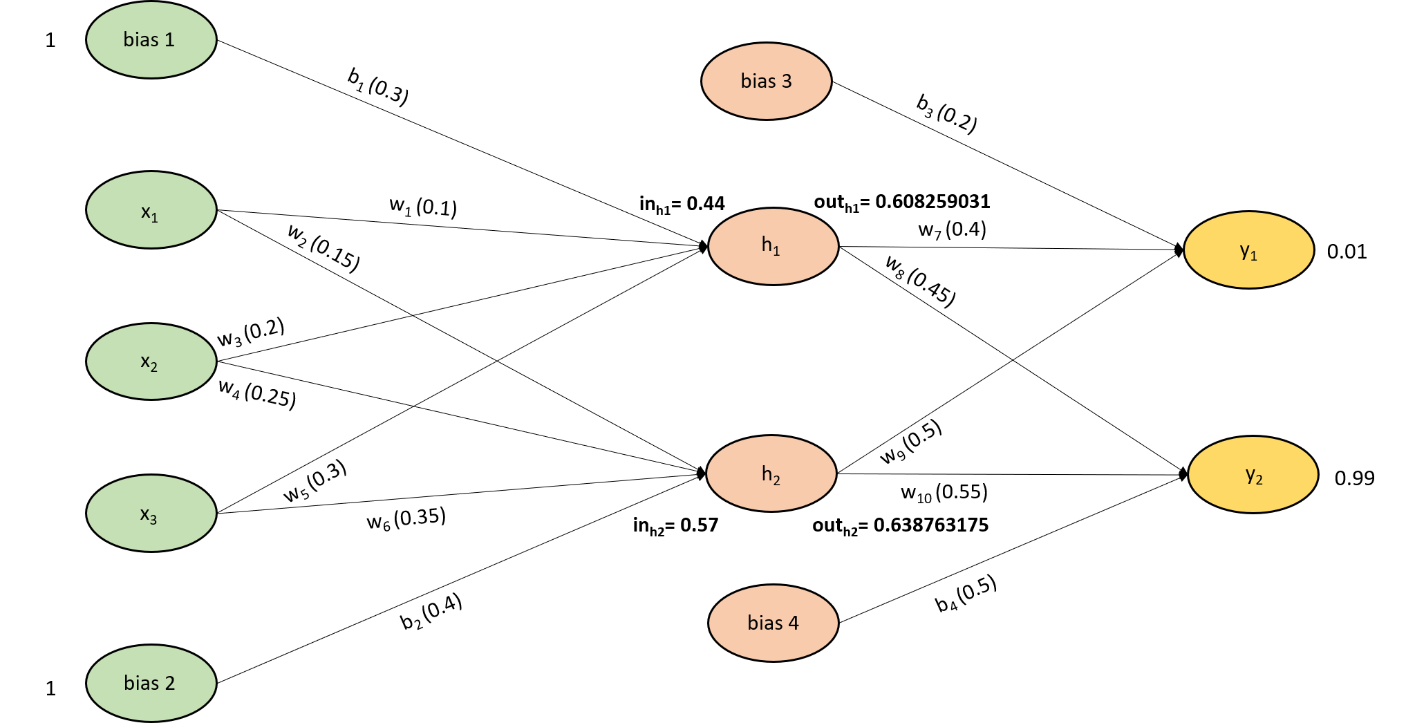
ii. Input and output at the output layer:
Now, let us calculate the input and output for the output layer neurons $y_1$ and $y_2$,
\[in_{y1}=w_7 * \text {out}_{h1}+w_9 * \text {out}_{h2}+b_3 * 1\] \[in_{y1}=0.4 * 0.608259031 +0.5 * 0.638763175+ 0.2 * 1\] \[in_{y1}=0.7626852\]with input 0.7626852, let us calculate the output from the neuron $y_1$,
\[out_{y1}=\frac{1}{1+e^{-in_{h1}}}=\frac{1}{1+e^{-0.0.7626852}}=0.681936436\]similarly, let us calculate for neuron $y_2$,
\[in_{y2}=w_8 * \text {out}_{h1}+w_{10} * \text {out}_{h2}+b_4 * 1\] \[in_{y2}=0.45 * 0.60825903 +0.55 * 0.63876318+ 0.5 * 1\] \[in_{y2}=1.12503631\]with input 1.12503631, let us calculate the output from the neuron $y_2$,
\[out_{y2}=\frac{1}{1+e^{-in_{h2}}}=\frac{1}{1+e^{-1.12503631}}=0.754921705\]
iii. Calculation of total error:
Now we have the predicted outputs from both the output layer neurons, hence now we can calculate the error for each output layer neuron to get the total error of the MLP.
\[Error_{\text {total}}=error_{y1} + error_{y2}\] \[Error_{\text {total}}=\frac{1}{2}\left(\text{target}_{y1}-\text{out}_{y1}\right)^2 + \frac{1}{2}\left(\text {target}_{y2}-\text {out}_{y2}\right)^2\] \[Error_{\text {total}}=\frac{1}{2}(0.01-0.681936436)^2 + \frac{1}{2}(0.99-0.754921705)^2\]\begin{equation} Error_{\text{total}}= 0.253380189 \label{eq:1} \end{equation}
2. Backpropagation:
The Backpropagation step in MLPs allows the network to learn from errors by adjusting weights and biases. This step propagates the error backward by updating weights and biases at each layer to minimize the difference between predicted and actual outputs. This process allows the network to make predictions or classify input data based on the learned patterns and connections between neurons. The chain rule of calculus is used in backpropagation efficiently to compute the gradient of the loss function at each layer, enabling accurate error calculation by all the weights and biases. This process can divided into the following steps
- Network error calculation: The output predicted from the network is compared with the actual output to calculate the total network error.
- Computation of gradients and weights and biases updation: The gradient of the error with respect to the weights and biases of the output layer is calculated, representing the direction and magnitude of the weight and bias modification needed to reduce the error. An optimization algorithm, such as gradient descent, will be used to update the weights and biases to reduce the error.
- Updation of parameters: The output layer weights and biases are updated using an optimization algorithm, such as gradient descent, which utilizes the calculated gradients to minimize the error iteratively.
- Propagation of error: The error information will be propagated backward to the previous layer by computing the error gradient with respect to the weights and biases of the previous layer. The weights and biases of the previous layer are modified using the calculated gradients with the gradient descent optimization algorithm.
- Iteration: Steps 4 is repeated for all hidden layers until the input layer is reached.
To summarize, the forward propagation is used to calculate the error, and the backpropagation is used to update network parameters so that the error during the subsequent forward propagation will be less than the current error. During the training of MLP, both forward and back propagation will be done in a continuous loop for a specified number of times (epoch) to optimize the model parameters so that the error at the end will be significantly less compared to the first epoch error.
The total error from the MLP with current weights and bias is 0.253380189, so let us calculate the optimized value for weights and bias using backpropagation with a learning rate of 0.5, so that error from MLP will be lesser than the current total error. In order to do that, we shall start with the weights ($w_7, w_8, w_9, w_{10}$) and biases ($b_3, b_4$) associated between the hidden layer and the output layer.
i. Weights between output and hidden layer:
Considering the weight $w_7$, first let us calculate the rate at which total error changes for the change in $w_7$,
\begin{equation} \frac{\partial E_{\text {total}}}{\partial w_7}=\frac{\partial E_{\text {total}}}{\partial out_{y1}} * \frac{\partial out_{y1}}{\partial in_{y1}} * \frac{\partial in_{y1}}{\partial w_7} \label{eq:2} \end{equation}
so, let us calculate the first component $\frac{\partial E_{\text {total}}}{\partial out_{y1}}$ in the equation \eqref{eq:2},
\[E_{\text {total}}=\frac{1}{2}\left(\text{target}_{y1}-\text {out}_{y1}\right)^2+\frac{1}{2}\left(\text {target}_{y2}-\text {out}_{y2}\right)^2\] \[\frac{\partial E_{\text {total}}}{\partial out_{y1}} = 2 * \frac{1}{2}\left(\text {target }_{y1}-\text {out}_{y1}\right)^{2-1} *-1+0\] \[\frac{\partial E_{\text {total}}}{\partial \text {out}_{y1}} = -\left(\text {target}_{y1}-\text {out}_{y1}\right)\] \[\frac{\partial E_{\text {total}}}{\partial \text {out}_{y1}} = - (0.01-0.681936436)\]\begin{equation} \frac{\partial E_{\text {total}}}{\partial \text {out}_{y1}} = 0.671936436 \label{eq:3} \end{equation}
the second component $\frac{\partial out_{y1}}{\partial in_{y1}}$ in the equation \eqref{eq:2} will be,
\[out_{y1}=\frac{1}{1+e^{-in_{y1}}}\] \[\frac{\partial out_{\text {y1}}}{\partial in_{y1}} = out_{y1} (1-out_{y1})\] \[\frac{\partial out_{\text {y1}}}{\partial in_{y1}} = 0.68193644 *(1-0.68193644)\]\begin{equation} \frac{\partial out_{\text {y1}}}{\partial in_{y1}} = 0.216899133 \label{eq:4} \end{equation}
the final component $\frac{\partial in_{\text {y1}}}{\partial \text{w}_{7}}$ in the equation \eqref{eq:2} will be,
\[in_{y1}=w_7 * \text {out}_{h1}+w_9 * \text {out}_{h2}+b_3 * 1\] \[\frac{\partial in_{\text {y1}}}{\partial \text{w}_{7}} = 1* \text {out}_{h1} * w_7^{(1-1)} + 0 + 0\] \[\frac{\partial in_{\text {y1}}}{\partial \text{w}_{7}} = out_{h1}\]\begin{equation} \frac{\partial in_{\text {y1}}}{\partial \text{w}_{7}} = 0.608259031 \label{eq:5} \end{equation}
let us take the values from equations \eqref{eq:3}, \eqref{eq:4}, and \eqref{eq:5} to calculate $\frac{\partial E_{\text {total}}}{\partial \text {w}_{7}}$ in the equation \eqref{eq:2}
\[\frac{\partial E_{\text {total}}}{\partial \text {w}_{7}} = 0.671936436 * 0.21689913 * 0.608259031 = 0.08864915\]once we calculate the rate at which total error changes for the change in $w_7$, the weight update rule to calculate the new optimized value for $w_7$ is as follows,
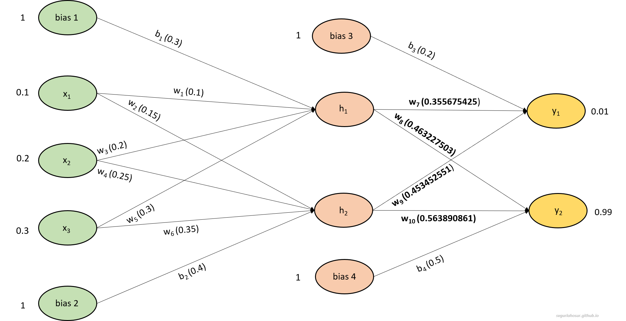
\[w_{7_{new}}= w_7 - \alpha \frac{\partial E_{\text {total}}}{\partial \text {w}_{7}}\] \[w_{7_{new}}= 0.4 - 0.5(0.08864915)\]\begin{equation} w_{7_{new}}= 0.355675425 \label{eq:6} \end{equation}
Now, similarly let us consider weight $w_9$, and calculate the rate at which total error changes for the change in $w_9$,
\begin{equation} \frac{\partial E_{\text {total}}}{\partial w_9}=\frac{\partial E_{\text {total}}}{\partial out_{y1}} * \frac{\partial out_{y1}}{\partial in_{y1}} * \frac{\partial in_{y1}}{\partial w_9} \label{eq:7} \end{equation}
considering the equation \eqref{eq:3}, the first component in equation \eqref{eq:7} is $\frac{\partial E_{\text {total}}}{\partial \text {out}_{y1}}=0.671936436$
and according to equation \eqref{eq:4} the second component in equation \eqref{eq:7} is $\frac{\partial out_{\text {y1}}}{\partial in_{y1}} =0.216899133$
the final component $\frac{\partial in_{\text {y1}}}{\partial \text {w}_{9}}$ in the equation \eqref{eq:7} will be as follows,
\[in\text{}_{y1}=w_7 * \text {out}_{h1}+w_9 * \text {out}_{h2}+b_3 * 1\] \[\frac{\partial in_{\text {y1}}}{\partial \text {w}_{9}} = 0 + 1* \text {out}_{h2} * w_9^{(1-1)}+ 0\] \[\frac{\partial in_{\text {y1}}}{\partial \text {w}_{9}} = out_{h2}\]\begin{equation} \frac{\partial in_{\text {y1}}}{\partial \text {w}_{9}} = 0.638763175 \label{eq:8} \end{equation}
so taking the values from equations \eqref{eq:3}, \eqref{eq:4}, and \eqref{eq:8} let us calculate $\frac{\partial E_{\text {total}}}{\partial \text {w}_{9}}$ in equation \eqref{eq:7}
\[\frac{\partial E_{\text {total}}}{\partial \text {w}_{9}} = 0.671936436 * 0.216899133 * 0.638763175 = 0.093094898\]once we calculate the rate at which total error changes for the change in $w_9$, the weight update rule to calculate the new optimized value for $w_9$ is as follows,
\[w_{9_{new}}= w_9 - \alpha \frac{\partial E_{\text {total}}}{\partial \text {w}_{9}}\] \[w_{9_{new}} = 0.5 - 0.5(0.093094898) = 0.453452551\]\begin{equation} w_{9_{new}}= 0.453452551 \label{eq:9} \end{equation}
Let us consider weight $w_8$, and calculate the rate at which total error changes for the change in $w_8$,
\begin{equation} \frac{\partial E_{\text {total}}}{\partial w_8}=\frac{\partial E_{\text {total}}}{\partial out_{y2}} * \frac{\partial out_{y2}}{\partial in_{y2}} * \frac{\partial in_{y2}}{\partial w_8} \label{eq:10} \end{equation}
so, let us calculate the first component $\frac{\partial E_{\text {total}}}{\partial out_{y2}}$ in the equation \eqref{eq:10},
\[E_{\text {total}}=\frac{1}{2}\left(\text {target}_{y1}-\text {out}_{y1}\right)^2+\frac{1}{2}\left(\text { target }_{y2}-\text { out }_{y2}\right)^2\] \[\frac{\partial E_{\text {total}}}{\partial out_{y2}} = 0 + 2 * \frac{1}{2}\left(\text {target}_{y2}-\text { out }_{y2}\right)^{2-1} *-1\] \[\frac{\partial E_{\text {total}}}{\partial \text {out}_{y2}}=-\left(\text {target}_{y2}-\text {out}_{y2}\right)\] \[\frac{\partial E_{\text {total}}}{\partial \text {out}_{y2}}= -(0.99-0.754921705)\]\begin{equation} \frac{\partial E_{\text {total}}}{\partial \text {out}_{y2}} = -0.235078295 \label{eq:11} \end{equation}
the second component $\frac{\partial out_{y2}}{\partial in_{y2}}$ in the equation \eqref{eq:10} will be,
\[out_{y2}=\frac{1}{1+e^{-in_{h2}}}\] \[\frac{\partial out_{\text {y2}}}{\partial in_{y2}} = out_{y2} (1-out_{y2})\] \[\frac{\partial out_{\text {y2}}}{\partial in_{y2}} = 0.754921705 *(1-0.754921705)\]\begin{equation} \frac{\partial out_{\text {y2}}}{\partial in_{y2}} = 0.185014924 \label{eq:12} \end{equation}
the final component $\frac{\partial in_{y2}}{\partial w_8}$ in the equation \eqref{eq:10} will be,
\[in_{y2}=w_8 * \text {out}_{h1}+w_{10} * \text {out}_{h2}+b_4 * 1\] \[\frac{\partial in_{\text {y2}}}{\partial \text {w}_{8}} = 1* \text {out}_{h1} * w_8^{(1-1)}+ 0 + 0\] \[\frac{\partial in_{\text {y2}}}{\partial \text {w}_{8}} = out_{h1}\]\begin{equation} \frac{\partial in_{\text {y2}}}{\partial \text {w}_{8}} = 0.608259031 \label{eq:13} \end{equation}
let us take the values from equations \eqref{eq:11}, \eqref{eq:12}, and \eqref{eq:13} to calculate $\frac{\partial E_{\text {total}}}{\partial \text {w}_{8}}$ in equation \eqref{eq:10}
\[\frac{\partial E_{\text {total}}}{\partial \text {w}_{8}} = -0.235078295 * 0.185014924 * 0.608259031 = -0.026455006\]once we calculate the rate at which total error changes for the change in $w_8$, the weight update rule to calculate the new optimized value for $w_8$ is as follows,
\[w_{8_{new}}= w_8 - \alpha \frac{\partial E_{\text {total}}}{\partial \text {w}_{8}}\] \[w_{8_{new}}= 0.45 - 0.5(-0.026455006)\]\begin{equation} w_{8_{new}}= 0.463227503 \label{eq:14} \end{equation}
Similarly, let us consider weight $w_{10}$, and calculate the rate at which total error changes for the change in $w_{10}$,
\begin{equation} \frac{\partial E_{\text {total}}}{\partial w_{10}}=\frac{\partial E_{\text {total}}}{\partial out_{y2}} * \frac{\partial out_{y2}}{\partial in_{y2}} * \frac{\partial in_{y2}}{\partial w_{10}} \label{eq:15} \end{equation}
considering the equation \eqref{eq:11}, the first component in equation \eqref{eq:15} is $\frac{\partial E_{\text {total}}}{\partial \text {out}_{y2}}=-0.235078295$
and according to equation \eqref{eq:12} the second component in equation \eqref{eq:15} is $\frac{\partial out_{\text {y2}}}{\partial in_{y2}} =0.185014924$
the final component $\frac{\partial in_{\text {y1}}}{\partial \text {w}_{10}}$ in equation \eqref{eq:15} will be as follows,
\[in_{y2}=w_8 * \text{out}_{h1}+w_{10} * \text {out}_{h2}+b_4 * 1\] \[\frac{\partial in_{\text {y2}}}{\partial \text {w}_{10}} = 0 + 1* \text {out}_{h2} * w_{10}^{(1-1)}+ 0\] \[\frac{\partial in_{\text {y2}}}{\partial \text {w}_{10}} = out_{h2}\]\begin{equation} \frac{\partial in_{\text {y2}}}{\partial \text {w}_{10}} = 0.638763175 \label{eq:16} \end{equation}
let us take values from equations \eqref{eq:8}, \eqref{eq:9}, and \eqref{eq:12} to calculate $\frac{\partial E_{\text {total}}}{\partial \text {w}_{10}}$ in equation \eqref{eq:15}
\[\frac{\partial E_{\text {total}}}{\partial \text {w}_{10}} = -0.235078295 * 0.185014924 * 0.638763175 = -0.027781722\]once we calculate the rate at which total error changes for the change in $w_{10}$, the weight update rule to calculate the new optimized value for $w_{10}$ is as follows,
\[w_{10_{new}}= w_{10} - \alpha \frac{\partial E_{\text {total}}}{\partial \text {w}_{10}}\] \[w_{10_{new}}= 0.55 - 0.5(-0.027781722) = 0.563890861\]\begin{equation} w_{10_{new}}= 0.563890861 \label{eq:17} \end{equation}
We have calculated all the weights ($w_7, w_8, w_9, w_{10}$) associated between the hidden layer and output layer.
ii. Biases between output and hidden layer:
Now let us calculate the biases ($b_3,b_4$) associated between the hidden layer and output layer. Considering the weight $b_{3}$, let us calculate the rate at which total error changes for the change in $b_{3}$,
\begin{equation} \frac{\partial E_{\text {total}}}{\partial b_3}=\frac{\partial E_{\text {total}}}{\partial out_{y1}} * \frac{\partial out_{y1}}{\partial in_{y1}} * \frac{\partial in_{y1}}{\partial b_3} \label{eq:18} \end{equation}
considering the equation \eqref{eq:3}, the first component in equation \eqref{eq:18} is $\frac{\partial E_{\text {total}}}{\partial \text {out}_{y1}}=0.671936436$
and according to equation \eqref{eq:4} the second component in equation \eqref{eq:18} is $\frac{\partial out_{\text {y1}}}{\partial in_{y1}} =0.216899133$
the final component $\frac{\partial in_{\text {y1}}}{\partial \text {b}_{3}}$ in equation \eqref{eq:18} will be as follows,
\[in\text{}_{y1}=w_7 * \text {out}_{h1}+w_9 * \text {out}_{h2}+b_3 * 1\] \[\frac{\partial in_{\text {y1}}}{\partial \text {b}_{3}} = 0 + 0 + 1\]\begin{equation} \frac{\partial in_{\text {y1}}}{\partial \text {b}_{3}} = 1 \label{eq:19} \end{equation}
so taking the values from \eqref{eq:3}, \eqref{eq:4}, and \eqref{eq:19} let us calculate $\frac{\partial E_{\text {total}}}{\partial \text {b}_{3}}$ in equation \eqref{eq:18}
\[\frac{\partial E_{\text {total}}}{\partial \text {b}_{3}} = 0.671936436 * 0.216899133 * 1 = 0.145742431\]once we calculate the rate at which total error changes for the change in $b_3$, the weight update rule to calculate the new optimized value for $b_3$ is as follows,
\[b_{3_{new}}= w_9 - \alpha \frac{\partial E_{\text {total}}}{\partial \text {b}_{3}}\] \[b_{3_{new}} = 0.2 - 0.5(0.145742431)\]\begin{equation} b_{3_{new}}= 0.127128785 \label{eq:20} \end{equation}
Similarly, let us consider weight $b_{4}$, and calculate the rate at which total error changes for the change in $b_{4}$,
\begin{equation} \frac{\partial E_{\text {total}}}{\partial b_{4}}=\frac{\partial E_{\text {total}}}{\partial out_{y2}} * \frac{\partial out_{y2}}{\partial in_{y2}} * \frac{\partial in_{y2}}{\partial b_{4}} \label{eq:21} \end{equation}
considering the equation \eqref{eq:11}, the first component in equation \eqref{eq:21} is $\frac{\partial E_{\text {total}}}{\partial \text {out}_{y2}}=-0.235078295$
and according to equation \eqref{eq:12} the second component in equation \eqref{eq:21} is $\frac{\partial out_{\text {y2}}}{\partial in_{y2}} =0.185014924$
the final component $\frac{\partial in_{\text {y1}}}{\partial \text {b}_{4}}$ in equation \eqref{eq:21} will be as follows,
\[in_{y2}=w_8 * \text{out}_{h1}+w_{10} * \text {out}_{h2}+b_4 * 1\] \[\frac{\partial in_{\text {y2}}}{\partial \text {b}_{4}} = 0 + 0 + 1\]\begin{equation} \frac{\partial in_{\text {y2}}}{\partial \text {b}_{4}} = 1 \label{eq:22} \end{equation}
let us take the values from equations \eqref{eq:11},\eqref{eq:12}, and \eqref{eq:22} to calculate $\frac{\partial E_{\text {total}}}{\partial \text {b}_{4}}$ in equation \eqref{eq:21}
\[\frac{\partial E_{\text {total}}}{\partial \text {b}_{4}} = -0.235078295 * 0.185014924 * 1 = -0.043492993\]once we calculate the rate at which total error changes for the change in $b_{4}$, the weight update rule to calculate the new optimized value for $b_{4}$ is as follows,
\[b_{4_{new}}= b_{4} - \alpha \frac{\partial E_{\text {total}}}{\partial \text {b}_{4}}\] \[b_{4_{new}}= 0.5 - 0.5(-0.043492993)\]\begin{equation} b_{4_{new}}= 0.521746497 \label{eq:23} \end{equation}
All the weights and bias values associated between the hidden layer and the output layer are calculated.

iii. Weights between hidden and input layer:
Now let us calculate the weights ($w_1, w_2, w_3, w_4, w_5, w_6$) and biases ($b_1, b_2$) associated between the hidden layer and input layer. Considering the weight $w_1$, first let us calculate the rate at which total error changes for the change in $w_1$,
\begin{equation} \frac{\partial E_{\text {total}}}{\partial w_1}=\frac{\partial E_{\text {total}}}{\partial out_{h1}} * \frac{\partial out_{h1}}{\partial in_{h1}} * \frac{\partial in_{h1}}{\partial w_1} \label{eq:24} \end{equation}
so, let us calculate the first component $\frac{\partial E_{\text {total}}}{\partial out_{h1}}$ in equation \eqref{eq:24}
\begin{equation} \frac{\partial E_{\text {total}}}{\partial out_{h1}} = \frac{\partial error_{\text {y1}}}{\partial out_{h1}} +\frac{\partial error_{\text {y2}}}{\partial out_{h1}} \label{eq:25} \end{equation}
the $\frac{\partial error_{\text {y1}}}{\partial out_{h1}}$ in equation \eqref{eq:25} has inturn two components as follows,
\begin{equation} \frac{\partial error_{\text {y1}}}{\partial out_{h1}} = \frac{\partial error_{\text {y1}}}{\partial in_{y1}} * \frac{\partial in_{\text {y1}}}{\partial out_{h1}} \label{eq:26} \end{equation}
the first component in equation \eqref{eq:26} is $\frac{\partial error_{\text {y1}}}{\partial in_{y1}} = \frac{\partial error_{\text {y1}}}{\partial out_{y1}} * \frac{\partial out_{\text {y1}}}{\partial in_{y1}}$ and by considering equations \eqref{eq:2} and \eqref{eq:3}
\begin{equation} \frac{\partial error_{\text {y1}}}{\partial in_{y1}} = 0.671936436 * 0.216899133 = 0.145742431 \label{eq:27} \end{equation}
the second component $\frac{\partial in_{\text {y1}}}{\partial out_{h1}}$ in equation \eqref{eq:26} will be as,
\[in_{y1}=w_7 * \text {out}_{h1}+w_9 * \text {out}_{h2}+b_3 * 1\]\begin{equation} \frac{\partial in_{\text {y1}}}{\partial out_{h1}} = w_7 = 0.4 \label{eq:28} \end{equation}
let us substitute values from the equation \eqref{eq:27} and \eqref{eq:28} in to equation \eqref{eq:26} \begin{equation} \frac{\partial error_{\text {y1}}}{\partial out_{h1}} = \frac{\partial error_{\text {y1}}}{\partial in_{y1}} * \frac{\partial in_{\text {y1}}}{\partial out_{h1}} = 0.145742431 * 0.4 = 0.058296972 \label{eq:29} \end{equation}
similarly the $\frac{\partial error_{\text {y2}}}{\partial out_{h1}}$ in \eqref{eq:25} also has inturn two components as follows,
\begin{equation} \frac{\partial error_{\text {y2}}}{\partial out_{h1}} = \frac{\partial error_{\text {y2}}}{\partial in_{y2}} * \frac{\partial in_{\text {y2}}}{\partial out_{h1}} \label{eq:30} \end{equation}
the first component in equation \eqref{eq:30} is $\frac{\partial error_{\text {y2}}}{\partial in_{y2}} = \frac{\partial error_{\text {y2}}}{\partial out_{y2}} * \frac{\partial out_{\text {y2}}}{\partial in_{y2}}$ and by considering the equation \eqref{eq:11} and \eqref{eq:12}
\begin{equation} \frac{\partial error_{\text {y2}}}{\partial in_{y2}} = −0.235078295 * 0.185014924 = -0.043492993 \label{eq:31} \end{equation}
the second component $\frac{\partial in_{\text {y2}}}{\partial out_{h1}}$ in the equation \eqref{eq:29} will be as,
\[in_{y2}=w_8 * \text {out}_{h1}+w_{10} * \text {out}_{h2}+b_4 * 1\]\begin{equation} \frac{\partial in_{\text {y2}}}{\partial out_{h1}} = w_8 = 0.45 \label{eq:32} \end{equation}
let us substitute values from the equations \eqref{eq:31} and \eqref{eq:32} in to equation \eqref{eq:30}
\begin{equation} \frac{\partial error_{\text {y2}}}{\partial out_{h1}} = \frac{\partial error_{\text {y2}}}{\partial in_{y2}} * \frac{\partial in_{\text {y2}}}{\partial out_{h1}} = -0.043492993 * 0.45 = -0.019571847 \label{eq:33} \end{equation}
now let us use the values from the equations \eqref{eq:29} and \eqref{eq:33} and substitute into equation \eqref{eq:25} which is the first component of the equation \eqref{eq:24}
\[\frac{\partial E_{\text {total}}}{\partial out_{h1}} = \frac{\partial error_{\text {y1}}}{\partial out_{h1}} +\frac{\partial error_{\text {y2}}}{\partial out_{h1}} = 0.058296972 + (-0.019571847)\]\begin{equation} \frac{\partial E_{\text {total}}}{\partial out_{h1}} = 0.038725125 \label{eq:34} \end{equation}
now let us calculate the second component $\frac{\partial out_{\text {h1}}}{\partial in_{h1}}$ of the equation \eqref{eq:24}
\[out_{h1}=\frac{1}{1+e^{-in_{h1}}}\] \[\frac{\partial out_{\text {h1}}}{\partial in_{h1}} = out_{h1} (1-out_{h1})\] \[\frac{\partial out_{\text {h1}}}{\partial in_{h1}} = 0.608259031 *(1-0.608259031)\]\begin{equation} \frac{\partial out_{\text {h1}}}{\partial in_{h1}} = 0.238279982 \label{eq:35} \end{equation}
now let us calculate the final component $\frac{\partial in_{\text {h1}}}{\partial \text{w}_{1}}$ of the equation \eqref{eq:24}
\[in_{h1}=w_1 * x_1+w_3 * x_2+w_5 * x_3+b_1 * 1\]\begin{equation} \frac{\partial in_{\text {h1}}}{\partial \text{w}_{1}} = x_1 = 0.1 \label{eq:36} \end{equation}
let us put everything together now from equations \eqref{eq:34}, \eqref{eq:35}, and \eqref{eq:36} into the equation \eqref{eq:24}
\[\frac{\partial E_{\text {total}}}{\partial w_1}=\frac{\partial E_{\text {total}}}{\partial out_{h1}} * \frac{\partial out_{h1}}{\partial in_{h1}} * \frac{\partial in_{h1}}{\partial w_1} = 0.038725125 * 0.238279982 * 0.1 = 0.009227422\]once we calculate the rate at which total error changes for the change in $w_1$, the weight update rule to calculate the new optimized value for $w_1$ is as follows,
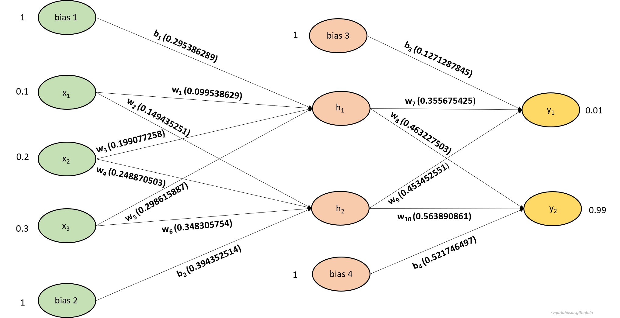
\[w_{1_{new}}= w_1 - \alpha \frac{\partial E_{\text {total}}}{\partial \text {w}_{1}}\] \[w_{1_{new}}= 0.1 - 0.5(0.000922742)\]\begin{equation} w_{1_{new}}= 0.099538629 \label{eq:37} \end{equation}
now, let us consider the weight $w_3$ and calculate the rate at which total error changes for the change in $w_3$,
\begin{equation} \frac{\partial E_{\text {total}}}{\partial w_3}=\frac{\partial E_{\text {total}}}{\partial out_{h1}} * \frac{\partial out_{h1}}{\partial in_{h1}} * \frac{\partial in_{h1}}{\partial w_3} \label{eq:38} \end{equation}
considering the equation \eqref{eq:34}, the first component in equation \eqref{eq:38} is $\frac{\partial E_{\text {total}}}{\partial out_{h1}} = 0.038725125$
and according to equation \eqref{eq:35} the second component in equation \eqref{eq:38} is $\frac{\partial out_{h1}}{\partial in_{h1}} = 0.238279982$
the final component $\frac{\partial in_{\text {h1}}}{\partial \text {w}_{3}}$ in the equation \eqref{eq:38} will be as follows,
\[in_{h1}=w_1 * x_1+w_3 * x_2+w_5 * x_3+b_1 * 1\]\begin{equation} \frac{\partial in_{\text {h1}}}{\partial \text{w}_{3}} = x_2 = 0.2 \label{eq:39} \end{equation}
so taking the values from equations \eqref{eq:34}, \eqref{eq:35}, and \eqref{eq:39} to calculate $\frac{\partial E_{\text {total}}}{\partial \text {w}_{3}}$ in the equation \eqref{eq:38}
\[\frac{\partial E_{\text {total}}}{\partial w_3}=\frac{\partial E_{\text {total}}}{\partial out_{h1}} * \frac{\partial out_{h1}}{\partial in_{h1}} * \frac{\partial in_{h1}}{\partial w_3} = 0.038725125 ∗ 0.238279982 ∗ 0.2 = 0.001845484\]once we calculate the rate at which total error changes for the change in $w_{3}$, the weight update rule to calculate the new optimized value for $w_{3}$ is as follows,
\[w_{3_{new}}= w_3 - \alpha \frac{\partial E_{\text {total}}}{\partial \text {w}_{3}}\] \[w_{3_{new}}= 0.2 - 0.5 * (0.08864915)\]\begin{equation} w_{3_{new}}= 0.199077258 \label{eq:40} \end{equation}
let us consider the weight $w_5$ and calculate the rate at which total error changes for the change in $w_5$,
\begin{equation} \frac{\partial E_{\text {total}}}{\partial w_5}=\frac{\partial E_{\text {total}}}{\partial out_{h1}} * \frac{\partial out_{h1}}{\partial in_{h1}} * \frac{\partial in_{h1}}{\partial w_5} \label{eq:41} \end{equation}
considering the equation \eqref{eq:34}, the first component in equation \eqref{eq:41} is $\frac{\partial E_{\text {total}}}{\partial out_{h1}} = 0.038725125$
and according to equation \eqref{eq:35} the second component in equation \eqref{eq:41} is $\frac{\partial out_{h1}}{\partial in_{h1}} = 0.238279982$
the final component $\frac{\partial in_{\text {h1}}}{\partial \text {w}_{5}}$ in equation \eqref{eq:41} will be as follows,
\[in_{h1}=w_1 * x_1+w_3 * x_2+w_5 * x_3+b_1 * 1\]\begin{equation} \frac{\partial in_{\text {h1}}}{\partial \text{w}_{5}} = x_3 = 0.3 \label{eq:42} \end{equation}
let us take values from the equations \eqref{eq:34}, \eqref{eq:35}, and \eqref{eq:42} to calculate $\frac{\partial E_{\text {total}}}{\partial \text {w}_{5}}$ in the equation \eqref{eq:41}
\[\frac{\partial E_{\text {total}}}{\partial w_5}=\frac{\partial E_{\text {total}}}{\partial out_{h1}} * \frac{\partial out_{h 1}}{\partial in_{h1}} * \frac{\partial in_{h1}}{\partial w_5} = 0.038725125 * 0.238279982 * 0.3 = 0.002768227\]once we calculate the rate at which total error changes for the change in $w_{5}$, the weight update rule to calculate the new optimized value for $w_{5}$ is as follows,
\[w_{5_{new}}= w_5 - \alpha \frac{\partial E_{\text {total}}}{\partial \text {w}_{5}}\] \[w_{5_{new}}= 0.3 - 0.5(0.002768227)\]\begin{equation} w_{5_{new}}= 0.298615887 \label{eq:43} \end{equation}
Considering the weight $w_2$, let us calculate the rate at which total error changes for the change in $w_2$
\begin{equation} \frac{\partial E_{\text {total}}}{\partial w_2}=\frac{\partial E_{\text {total}}}{\partial out_{h2}} * \frac{\partial out_{h2}}{\partial in_{h2}} * \frac{\partial in_{h2}}{\partial w_2} \label{eq:44} \end{equation}
so, let us calculate the first component $\frac{\partial E_{\text {total}}}{\partial out_{h2}}$ in the equation \eqref{eq:44}
\begin{equation} \frac{\partial E_{\text {total}}}{\partial out_{h2}} = \frac{\partial error_{\text {y1}}}{\partial out_{h2}} +\frac{\partial error_{\text {y2}}}{\partial out_{h2}} \label{eq:45} \end{equation}
the $\frac{\partial error_{\text {y1}}}{\partial out_{h2}}$ in the equation \eqref{eq:45} inturn has two components as follows,
\begin{equation} \frac{\partial error_{\text {y1}}}{\partial out_{h2}} = \frac{\partial error_{\text {y1}}}{\partial in_{y1}} * \frac{\partial in_{\text {y1}}}{\partial out_{h2}} \label{eq:46} \end{equation}
by considering the equation \eqref{eq:27} , the first component in equation \eqref{eq:46} is $\frac{\partial error_{\text {y1}}}{\partial in_{y1}} = 0.145742431$
the second component $\frac{\partial in_{\text {y1}}}{\partial out_{h2}}$ in the equation \eqref{eq:46} will be as,
\[in_{y1}=w_7 * \text {out}_{h1}+w_9 * \text {out}_{h2}+b_3 * 1\]\begin{equation} \frac{\partial in_{\text {y1}}}{\partial out_{h2}} = w_9 = 0.5 \label{eq:47} \end{equation}
let us substitute values from the equation \eqref{eq:27} and \eqref{eq:47} in to equation \eqref{eq:46}
\begin{equation} \frac{\partial error_{\text {y1}}}{\partial out_{h2}} = \frac{\partial error_{\text {y1}}}{\partial in_{y1}} * \frac{\partial in_{\text {y1}}}{\partial out_{h2}} = 0.145742431 * 0.5 = 0.072871216 \label{eq:48} \end{equation}
similarly the $\frac{\partial error_{\text {y2}}}{\partial out_{h2}}$ in the equation \eqref{eq:32} also has inturn two components as follows,
\begin{equation} \frac{\partial error_{\text {y2}}}{\partial out_{h2}} = \frac{\partial error_{\text {y2}}}{\partial in_{y2}} * \frac{\partial in_{\text {y2}}}{\partial out_{h2}} \label{eq:49} \end{equation}
by considering the equation \eqref{eq:31} the first component in the equation \eqref{eq:49} $\frac{\partial error_{\text {y2}}}{\partial in_{y2}} =−0.043492993$
the second component $\frac{\partial in_{\text {y2}}}{\partial out_{h2}}$ in the equation \eqref{eq:49} will be as,
\[in_{y2}=w_8 * \text {out}_{h1}+w_{10} * \text {out}_{h2}+b_4 * 1\]\begin{equation} \frac{\partial in_{\text {y2}}}{\partial out_{h2}} = w_{10} = 0.55 \label{eq:50} \end{equation}
let us substitute values from the equation \eqref{eq:48} and \eqref{eq:49} in to the equation \eqref{eq:49}
\[\frac{\partial error_{\text {y2}}}{\partial out_{h2}} = \frac{\partial error_{\text {y2}}}{\partial in_{y2}} * \frac{\partial in_{\text {y2}}}{\partial out_{h2}} = −0.043492993 * 0.55\] \[\frac{\partial error_{\text {y2}}}{\partial out_{h2}} = −0.043492993 * 0.55\]\begin{equation} \frac{\partial error_{\text {y2}}}{\partial out_{h2}} = -0.023921146 \label{eq:51} \end{equation}
let us use the values from equations \eqref{eq:48} and \eqref{eq:51} and substitute them into equation \eqref{eq:45} which is the first component of the equation \eqref{eq:44}
\[\frac{\partial E_{\text {total}}}{\partial out_{h2}} = \frac{\partial error_{\text {y1}}}{\partial out_{h2}} +\frac{\partial error_{\text {y2}}}{\partial out_{h2}} = 0.072871216 + (-0.023921146)\]\begin{equation} \frac{\partial E_{\text {total}}}{\partial out_{h2}} = 0.048950069 \label{eq:52} \end{equation}
now let us calculate the second component $\frac{\partial out_{\text {h2}}}{\partial in_{h2}}$ of the equation \eqref{eq:44}
\[out_{h2}=\frac{1}{1+e^{-in_{h2}}}\] \[\frac{\partial out_{\text {h2}}}{\partial in_{h2}} = out_{h2} (1-out_{h2})\] \[\frac{\partial out_{\text {h2}}}{\partial in_{h2}} = 0.638763175 *(1-0.638763175)\]\begin{equation} \frac{\partial out_{\text {h2}}}{\partial in_{h2}} = 0.230744781 \label{eq:53} \end{equation}
now let us calculate the final component $\frac{\partial in_{\text {h2}}}{\partial \text{w}_{2}}$ of the equation \eqref{eq:44}
\[in_{h2}=w_2 * x_1+w_4 * x_2+w_6 * x_3+b_2 * 1\]\begin{equation} \frac{\partial in_{\text {h2}}}{\partial \text{w}_{2}} = x_1 = 0.1 \label{eq:54} \end{equation}
let us put values from the from equations \eqref{eq:52}, \eqref{eq:53} and \eqref{eq:54} into the equation \eqref{eq:44}
\[\frac{\partial E_{\text {total}}}{\partial w_2}=\frac{\partial E_{\text {total}}}{\partial out_{h2}} * \frac{\partial out_{h2}}{\partial in_{h2}} * \frac{\partial in_{h2}}{\partial w_2} = 0.048950069 * 0.230744781 * 0.1 = 0.001129497\]once we calculate the rate at which total error changes for the change in $w_2$, the weight update rule to calculate the new optimized value for $w_2$ is as follows,
\[w_{2_{new}}= w_2 - \alpha \frac{\partial E_{\text {total}}}{\partial \text {w}_{2}}\] \[w_{2_{new}}= 0.15 - 0.5(0.001129497) = 0.149435251\]\begin{equation} w_{2_{new}}= 0.149435251 \label{eq:55} \end{equation}
let us consider the weight $w_4$ and calculate the rate at which total error changes for the change in $w_4$,
\begin{equation} \frac{\partial E_{\text {total }}}{\partial w_4}=\frac{\partial E_{\text {total }}}{\partial out_{h2}} * \frac{\partial out_{h2}}{\partial in_{h2}} * \frac{\partial in_{h2}}{\partial w_4} \label{eq:56} \end{equation}
considering equation \eqref{eq:52}, the first component in the equation \eqref{eq:56} is $\frac{\partial E_{\text {total}}}{\partial out_{h2}} = 0.048950069$
considering equation \eqref{eq:53}, the second component in the equation \eqref{eq:56} is $\frac{\partial out_{h2}}{\partial in_{h2}} = 0.230744781$
the final component $\frac{\partial in_{\text {h1}}}{\partial \text{w}_{4}}$ in the equation \eqref{eq:56} will be as follows,
\[in_{h2}=w_2 * x_1+w_4 * x_2+w_6 * x_3+b_2 * 1\]\begin{equation} \frac{\partial in_{\text {h1}}}{\partial \text{w}_{4}} = x_2 = 0.2 \label{eq:57} \end{equation}
let us take the values from \eqref{eq:52}, \eqref{eq:53} and \eqref{eq:57} to calculate $\frac{\partial E_{\text {total}}}{\partial w_4}$ in the equation \eqref{eq:56}
\[\frac{\partial E_{\text {total}}}{\partial w_4}=\frac{\partial E_{\text {total }}}{\partial out_{h2}} * \frac{\partial out_{h2}}{\partial in_{h2}} * \frac{\partial in_{h2}}{\partial w_4} = 0.048950069 ∗ 0.230744781 ∗ 0.2 = 0.002258995\]once we calculate the rate at which total error changes for the change in $w_4$, the weight update rule to calculate the new optimized value for $w_4$ is as follows,
\[w_{4_{new}}= w_4 - \alpha \frac{\partial E_{\text {total}}}{\partial \text {w}_{4}}\] \[w_{4_{new}}= 0.25 - 0.5(0.002258995)\]\begin{equation} w_{4_{new}}= 0.248870503 \label{eq:58} \end{equation}
let us consider the weight $w_6$ and calculate the rate at which total error changes for the change in $w_6$,
\begin{equation} \frac{\partial E_{\text {total}}}{\partial w_6}=\frac{\partial E_{\text {total}}}{\partial out_{h2}} * \frac{\partial out_{h2}}{\partial in_{h2}} * \frac{\partial in_{h2}}{\partial w_6} \label{eq:59} \end{equation}
considering equation \eqref{eq:52}, the first component in the equation \eqref{eq:59} is $\frac{\partial E_{\text {total}}}{\partial out_{h2}} = 0.048950069$
considering equation \eqref{eq:53}, the second component in the equation \eqref{eq:59} is $\frac{\partial out_{h2}}{\partial in_{h2}} = 0.230744781$
the final component $\frac{\partial in_{\text {h1}}}{\partial \text{w}_{6}}$ in the equation \eqref{eq:59} will be as follows,
\[in_{h2}=w_2 * x_1+w_4 * x_2+w_6 * x_3+b_2 * 1\]\begin{equation} \frac{\partial in_{\text {h2}}}{\partial \text{w}_{6}} = x_3 = 0.3 \label{eq:60} \end{equation}
let us take the values from the equations \eqref{eq:52}, \eqref{eq:53} and \eqref{eq:60} to calculate $\frac{\partial E_{\text {total}}}{\partial w_6}$ in the equation \eqref{eq:59}
\[\frac{\partial E_{\text {total}}}{\partial w_6}=\frac{\partial E_{\text {total}}}{\partial out_{h2}} * \frac{\partial out_{h2}}{\partial in_{h2}} * \frac{\partial in_{h2}}{\partial w_6} = 0.048950069 ∗ 0.230744781 ∗ 0.3 = 0.003388492\]once we calculate the rate at which total error changes for the change in $w_6$, the weight update rule to calculate the new optimized value for $w_6$ is as follows,
\[w_{6_{new}}= w_6 - \alpha \frac{\partial E_{\text {total}}}{\partial \text {w}_{6}}\] \[w_{6_{new}}= 0.35 - 0.5(0.003388492)\]\begin{equation} w_{6_{new}}= 0.348305754 \label{eq:61} \end{equation}
We have calculated all the weights ($w_1, w_2, w_3, w_4, w_5, w_6$) associated between the hidden layer and output layer.

iv. Biases between hidden and input layer:
Now let us calculate the biases ($b_1, b_2$) associated between the hidden layer and output layer. Considering the bias $b_1$, let us calculate the rate at which total error changes for the change in $b_1$,
\begin{equation} \frac{\partial E_{\text {total}}}{\partial b_1}=\frac{\partial E_{\text {total}}}{\partial out_{h1}} * \frac{\partial out_{h1}}{\partial in_{h1}} * \frac{\partial in_{h1}}{\partial b_1} \label{eq:62} \end{equation}
considering the equation \eqref{eq:34}, the first component in the equation \eqref{eq:62} is $\frac{\partial E_{\text {total}}}{\partial out_{h1}} = 0.038725125$
and according to equation \eqref{eq:35} the second component in the equation \eqref{eq:62} is $\frac{\partial out_{h1}}{\partial in_{h1}} = 0.238279982$
the final component $\frac{\partial in_{\text {h1}}}{\partial \text {b}_{1}}$ in the equation \eqref{eq:62} will be as follows,
\[in_{h1}=w_1 * x_1+w_3 * x_2+w_5 * x_3+b_1 * 1\]\begin{equation} \frac{\partial in_{\text {h1}}}{\partial \text{b}_{1}} = 0 * 0 * 1 = 1 \label{eq:63} \end{equation}
let us the values from the equations \eqref{eq:34}, \eqref{eq:35}, and \eqref{eq:63} to calculate $\frac{\partial E_{\text {total}}}{\partial \text {b}_{1}}$ in the equation \eqref{eq:62}
\[\frac{\partial E_{\text {total}}}{\partial b_1}=\frac{\partial E_{\text {total}}}{\partial out_{h1}} * \frac{\partial out_{h1}}{\partial in_{h1}} * \frac{\partial in_{h1}}{\partial b_1} = 0.038725125 ∗ 0.238279982 ∗ 1 = 0.009227422\]once we calculate the rate at which total error changes for the change in $b_{1}$, the weight update rule to calculate the new optimized value for $b_{1}$ is as follows,
\[b_{1_{new}}= b_1 - \alpha \frac{\partial E_{\text {total}}}{\partial \text {b}_{1}}\] \[b_{1_{new}}= 0.3 - 0.5 * (0.009227422)\]\begin{equation} b_{1_{new}}= 0.295386289 \label{eq:64} \end{equation}
now let us consider the bias $b_2$ and calculate the rate at which total error changes for the change in $b_2$,
\begin{equation} \frac{\partial E_{\text {total}}}{\partial b_2}=\frac{\partial E_{\text {total}}}{\partial out_{h2}} * \frac{\partial out_{h2}}{\partial in_{h2}} * \frac{\partial in_{h2}}{\partial b_2} \label{eq:65} \end{equation}
considering equation \eqref{eq:52}, the first component in the equation \eqref{eq:65} is $\frac{\partial E_{\text {total}}}{\partial out_{h2}} = 0.048950069$
considering equation \eqref{eq:53}, the second component in the equation \eqref{eq:65} is $\frac{\partial out_{h2}}{\partial in_{h2}} = 0.230744781$
the final component $\frac{\partial in_{\text {h1}}}{\partial \text{b}_{2}}$ in the equation \eqref{eq:65} will be as follows,
\[in_{h2}=w_2 * x_1+w_4 * x_2+w_6 * x_3+b_2 * 1\]\begin{equation} \frac{\partial in_{\text {h2}}}{\partial \text{b}_{2}} = 0 + 0 + 1 = 1 \label{eq:66} \end{equation}
let us take the values from the equations \eqref{eq:52}, \eqref{eq:53} and \eqref{eq:66} to calculate $\frac{\partial E_{\text {total}}}{\partial b_2}$ in the equation \eqref{eq:65}
\[\frac{\partial E_{\text {total}}}{\partial b_2}=\frac{\partial E_{\text {total}}}{\partial out_{h2}} * \frac{\partial out_{h2}}{\partial in_{h2}} * \frac{\partial in_{h2}}{\partial b_2} = 0.048950069 ∗ 0.230744781 ∗ 1 = 0.011294973\]once we calculate the rate at which total error changes for the change in $b_2$, the weight update rule to calculate the new optimized value for $b_2$ is as follows,
\[b_{2_{new}}= b_2 - \alpha \frac{\partial E_{\text {total}}}{\partial \text {b}_{2}}\] \[b_{2_{new}}= 0.4 - 0.5 * (0.011294973)\]\begin{equation} b_{2_{new}}= 0.394352514 \label{eq:67} \end{equation}
We have calculated all the biases ($b_1, b_2$) associated between the hidden layer and input layer.
3. Forward propagation with both updated weights and biases
First, let us calculate the input and outputs at the hidden layer neuron $h_1$ and $h_2$ with the given three inputs $x_1$, $x_2$, and $x_3$.
\[in_{h1}=w_1 * x_1+w_3 * x_2+w_5 * x_3+b_1 * 1\] \[in_{h1}=0.099538629 * 0.1+0.199077258 * 0.2+ 0.298615887 * 0.3 + 0.295386289 * 1\] \[in_{h1}=0.434740369\]with input 0.434740369, let us calculate the output from the neuron $h_1$,
\[out_{h1}=\frac{1}{1+e^{-input_{h1}}}=\frac{1}{1+e^{-0.434740369}}=0.607005055\]Similarly, let us calculate the input and output for the neuron for $h_2$,
\[in_{h2}=w_2 * x_1+w_4 * x_2+w_6 * x_3+b_2 * 1\] \[in_{h2}=0.149435251 * 0.1+0.248870503 * 0.2+ 0.348305754 * 0.3 + 0.394352514 * 1\] \[in_{h2}=0.563561865\]with input 0.563561865, let us calculate the output from the neuron $h_2$,
\[out_{h2}=\frac{1}{1+e^{-in_{h2}}}=\frac{1}{1+e^{-0.563561865}}=0.637276286\]Now, let us finally calculate the input and output for the neuron $y_1$ and $y_2$.
\[in_{y1}=w_7 * \text {out}_{h1}+w_9 * \text {out}_{h2}+b_3 * 1\] \[in_{y1}=0.355675425 * 0.607005055 +0.453452551 * 0.637276286+ 0.127128785 * 1\] \[in_{y1}=0.632000123\]with input 0.632000123, let us calculate the output from the neuron $y_1$,
\[out_{y1}=\frac{1}{1+e^{-in_{h1}}}=\frac{1}{1+e^{-0.632000123}}=0.652942846\]similarly, let us calculate for neuron $y_2$,
\[in_{y2}=w_8 * \text {out}_{h1}+w_{10} * \text {out}_{h2}+b_4 * 1\] \[in_{y2}=0.463227503 * 0.60810511 +0.563890861 * 0.638580717+ 0.521746497 * 1\] \[in_{y2}=1.162282206\]with input 1.162282206, let us calculate the output from the neuron $y_2$,
\[out_{y2}=\frac{1}{1+e^{-in_{h2}}}=\frac{1}{1+e^{-1.162282206}}=0.761747156\]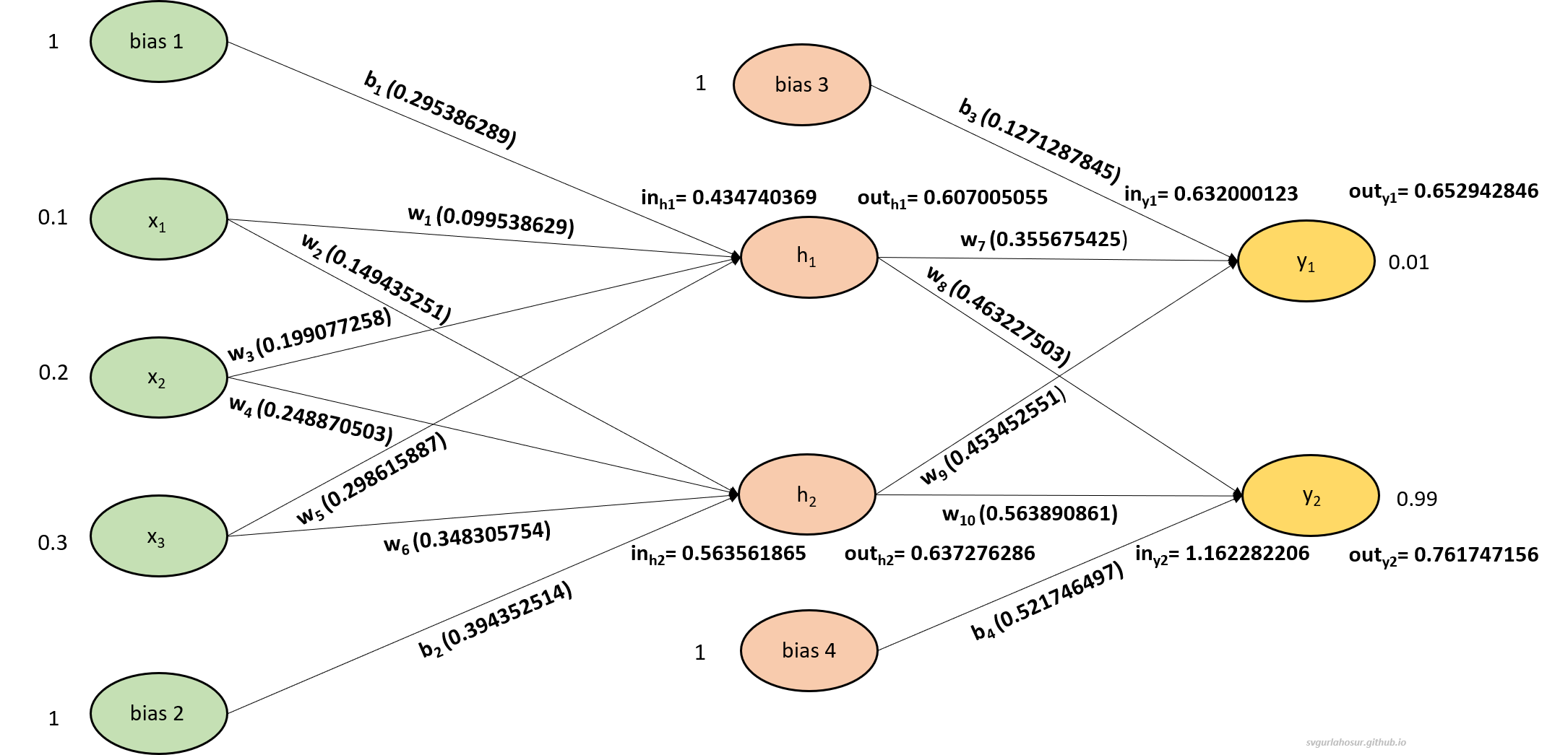
i. Calculation of total error:
Now we have the predicted outputs from both the output layer neurons, hence now we can calculate the error for each output layer neuron to get the total error of the MLP.
\[Error_{\text {total}}=error_{y1} + error_{y2}\] \[Error_{\text {total}}=\frac{1}{2}\left(\text{target}_{y1}-\text{out}_{y1}\right)^2 + \frac{1}{2}\left(\text {target}_{y2}-\text {out}_{y2}\right)^2\] \[Error_{\text {total}}=\frac{1}{2}(0.01-0.652942846)^2 + \frac{1}{2}(0.99-0.761747156)^2\]\begin{equation} Error_{\text{total}}= 0.232737432 \label{eq:68} \end{equation}
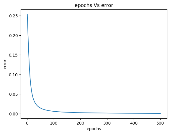
The total error from the MLP before the updation of weights and bias was $0.253380189$, and now the total error after one epoch is $0.232737432$, which is less than the original error. If we continue updating the weights and bias in an iterative loop for some particular number of epochs, the error eventually reduces, and the predicted output from the MLP will be closer to the actual outputs. The complete code for MLP, which does the updation of weights and bias during backpropagation, is as follows.
Epoch: 50 Error: 0.014331249
Epoch: 100 Error: 0.005898502
Epoch: 150 Error: 0.003500656
Epoch: 200 Error: 0.002409748
Epoch: 250 Error: 0.001798825
Epoch: 300 Error: 0.001413341
Epoch: 350 Error: 0.001150407
Epoch: 400 Error: 0.000960931
Epoch: 450 Error: 0.000818692
Epoch: 500 Error: 0.000708482
4. Forward propagation with only updated weights:
First, let us calculate the input and outputs at the hidden layer neuron $h_1$ and $h_2$ with the given three inputs $x_1$, $x_2$, and $x_3$.
\[in_{h1}=w_1 * x_1+w_3 * x_2+w_5 * x_3+b_1 * 1\] \[in_{h1}=0.099538629 * 0.1+0.199077258 * 0.2+ 0.298615887 * 0.3 + 0.3 * 1\] \[in_{h1}=0.43935408\]with input 0.43935408, let us calculate the output from the neuron $h_1$,
\[out_{h1}=\frac{1}{1+e^{-input_{h1}}}=\frac{1}{1+e^{-0.43935408}}=0.60810511\]Similarly, let us calculate the input and output for the neuron for $h_2$,
\[in_{h2}=w_2 * x_1+w_4 * x_2+w_6 * x_3+b_2 * 1\] \[in_{h2}=0.149435251 * 0.1+0.248870503 * 0.2+ 0.348305754 * 0.3 + 0.4 * 1\] \[in_{h2}=0.569209352\]with input 0.569209352, let us calculate the output from the neuron $h_2$,
\[out_{h2}=\frac{1}{1+e^{-in_{h2}}}=\frac{1}{1+e^{-0.569209352}}=0.638580717\]Now, let us finally calculate the input and output for the neuron $y_1$ and $y_2$.
\[in_{y1}=w_7 * \text {out}_{h1}+w_9 * \text {out}_{h2}+b_3 * 1\] \[in_{y1}=0.355675425 * 0.60810511 +0.453452551 * 0.638580717+ 0.2 * 1\] \[in_{y1}=0.705854099\]with input 0.705854099, let us calculate the output from the neuron $y_1$,
\[out_{y1}=\frac{1}{1+e^{-in_{h1}}}=\frac{1}{1+e^{-0.705854099}}=0.669484421\]similarly, let us calculate for neuron $y_2$,
\[in_{y2}=w_8 * \text {out}_{h1}+w_{10} * \text {out}_{h2}+b_4 * 1\] \[in_{y2}=0.463227503 * 0.60810511 +0.563890861 * 0.638580717+ 0.5 * 1\] \[in_{y2}=1.141780842\]with input 1.141780842, let us calculate the output from the neuron $y_2$,
\[out_{y2}=\frac{1}{1+e^{-in_{h2}}}=\frac{1}{1+e^{-1.141780842}}=0.758006454\]
i. Calculation of total error:
Now we have the predicted outputs from both the output layer neurons, hence now we can calculate the error for each output layer neuron to get the total error of the MLP.
\[Error_{\text {total}}=error_{y1} + error_{y2}\] \[Error_{\text {total}}=\frac{1}{2}\left(\text{target}_{y1}-\text{out}_{y1}\right)^2 + \frac{1}{2}\left(\text {target}_{y2}-\text {out}_{y2}\right)^2\] \[Error_{\text {total}}=\frac{1}{2}(0.01-0.669484421)^2 + \frac{1}{2}(0.99-0.758006454)^2\]\begin{equation} Error_{\text{total}}= 0.244370353 \label{eq:69} \end{equation}
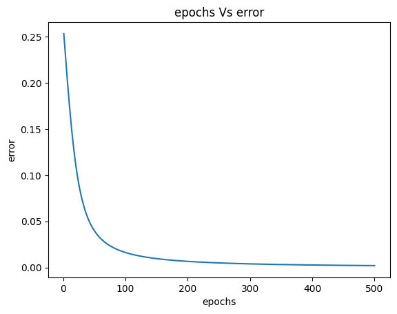
The total error from the MLP before the updation of weights was $0.253380189$, and the total error after one epoch is $0.244370353$, which is less than the original error. Still, it is more than the error obtained when we updated both weights and bias $0.232737432$. If we continue updating the weights in an iterative loop for some particular number of epochs, the error eventually reduces, and the predicted output from the MLP will be closer to the actual outputs. The complete code for MLP, which does the updation of only weights during backpropagation, is as follows.
Epoch: 50 Error: 0.039914599
Epoch: 100 Error: 0.016219482
Epoch: 150 Error: 0.009572182
Epoch: 200 Error: 0.006583904
Epoch: 250 Error: 0.00492128
Epoch: 300 Error: 0.003876254
Epoch: 350 Error: 0.003165179
Epoch: 400 Error: 0.002653526
Epoch: 450 Error: 0.002269746
Epoch: 500 Error: 0.001972481
5. Analysis on the error obtained during training:
Now, let us analyze the error obtained for both methods and visualize how error has reduced over the training. The following graph shows that the updation of the weights and biases method leads to better network convergence during gradient descent optimization. Hence, during MLP training, weights and biases should be updated through optimization techniques like gradient descent or backpropagation to minimize the loss function and improve the network’s performance since they are necessary to learn and generalize from the training data.
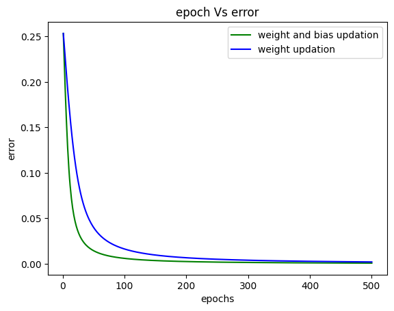
The total error from all epochs with weights and bias updation method is less.
6. References:
- Machine Learning, Tom Mitchell, McGraw Hill, 1997.
- “CS229: Machine Learning” course by Andrew N G at Stanford, Autumn 2018.
Leave a Comment