This post provides an in-detail discussion of the Logistic Regression algorithm with Real-World example and its implementation from scratch using Python.

Introduction

Logistic Regression is a Supervised Learning algorithm used to solve problems where for every input(X), the respective output (Y) values are always discrete in nature. To understand the Logistic Regression algorithm, let us look into some real-world problems solved with this algorithm’s help.

• Vehicle features and price –> Buy/ Do not buy
• Credit score of customer –> Loan scanctioned/ not
• Marks scored in entrance exam –> Admitted to university/ not

In all the examples, output/predicted values are discrete; hence, Logistic regression is used to build the machine learning model (hypothesis) and predict the output for a new set of inputs. To understand the algorithm from a practical perspective, let us take the problem of diagnostically predicting whether or not a patient has diabetes based on certain diagnostic measurements. To solve this problem with Logistic Regression, we should apply the following four steps:

1. Data collection
2. Model/hypothesis represenation
3. Cost calculation
4. Optimization of model parameters

1. Data Collection

Let us consider the dataset from the National Institute of Diabetes and Digestive and Kidney Diseases. The objective of the dataset is to diagnostically predict whether or not a patient has diabetes, based on certain diagnostic measurements included in the dataset. The datasets consists of several medical predictor variables/features(their BMI, insulin level, age, and so on) and one target variable/output(whether or not a patient has diabetes).

Note:

1. Number of samples(records) range from 1, 2, 3, 4, . . . ., m
2. Number of features range from $x_0, x_1, x_2, x_3, . . . . x_n$ where $x_0$ is considered as 1
3. Notation used to identify the dataset(superscript indicates the sample number and subscript indicates the feature number): $x^2$ - (1, 111, 62, 13, 182, 24, 0.138, 23), $x^2_1$ - 1, $x^2_2$ - 111 and $x^4$ - (3, 174, 58, 22, 194, 32.9, 0.593, 36)

Visit the training and testing for the complete data.

Since the dataset has eight features, and each feature has a different range of values, we need to normalize the values in the features for the dataset. The normalization process changes the values of all features in the dataset to a common scale without distorting differences in the ranges of values. The data normalization ensures that all features in a dataset are on a common scale, enabling fair comparisons and stable model performance during machine learning.

Several data normalization techniques include Min-Max Normalization, Z-Score Standardization, Log Transformation, Quantile Transformation, etc. Here, apply the Min-Max normalization, which rescales data to a specific range, typically between 0 and 1, by subtracting the minimum value and dividing by the range (max-min).

2. Model/hypothesis represenation

The model/hypothesis($h_\theta(x)$) approximates the target function by finding a relationship(pattern) between input and output. The hypothesis used in Linear regression($h_{\theta}(x)=\theta^{T}x$) cannot be utilized directly here since it predicts continuous values; we want it to be predicting discrete values and in the considered problem it is either ‘0’ or ‘1’. Hence we go for new hypothesis called sigmoid function($g\left(\theta^{T} x\right)$) also called a squashing function as its domain is the set of all real numbers, and its range is (0, 1).

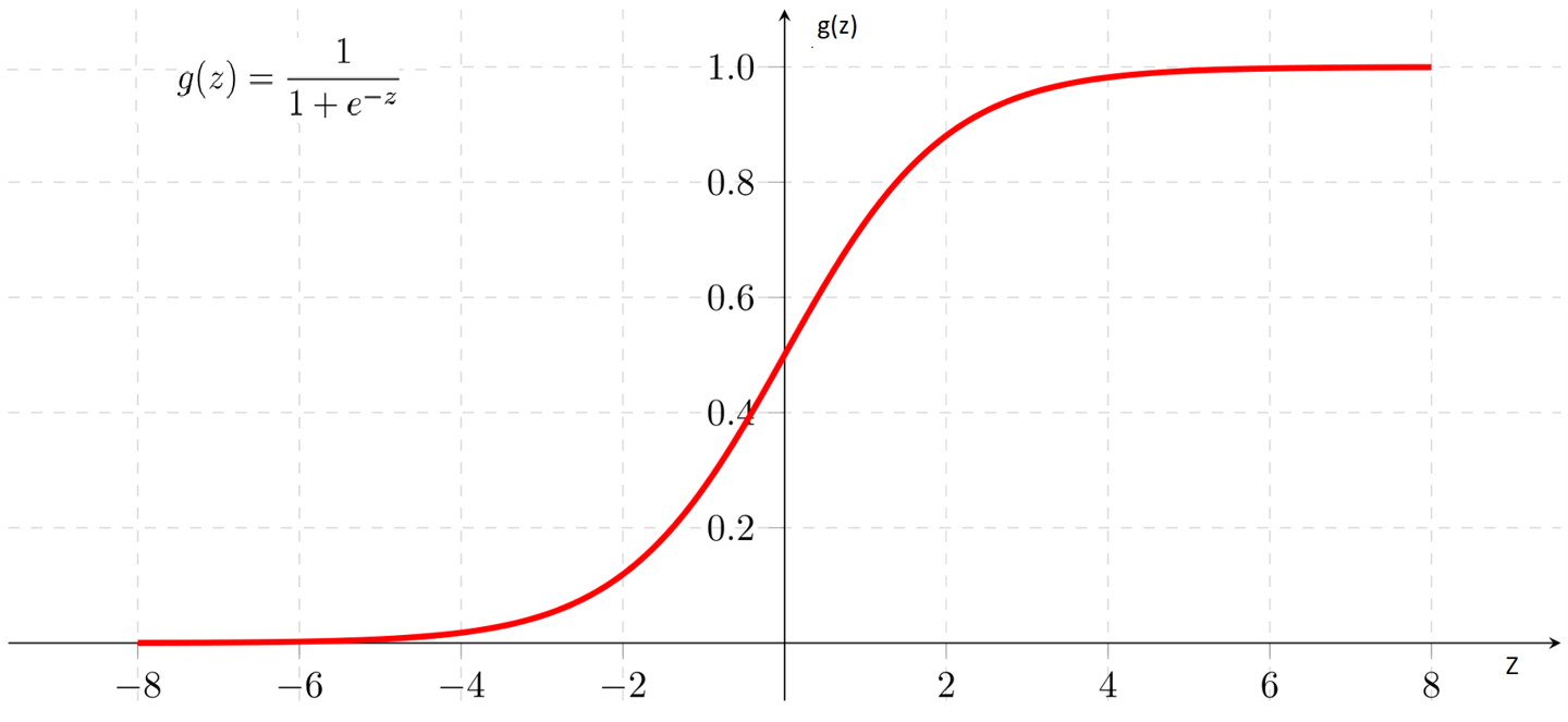
Hence, by using the sigmoid function as the hypothesis function $h_\theta(x) = g(z)$ , where z = $\theta^{T}x$,

now we can always ensure that values predicted by the hypothesis($h_\theta(x)$) is always \(0 \leq h_{\theta}(x) \leq 1\) and we also define one more new condition since we need output from hypothesis to have only two values either ‘0’ or ‘1’.

if \(h_\theta(x) \geq 0.5\), we will consider that \(h_\theta(x) = 1\)

else \(h_\theta(x) < 0.5\), we will consider that \(h_\theta(x) = 0\)

3. Cost function

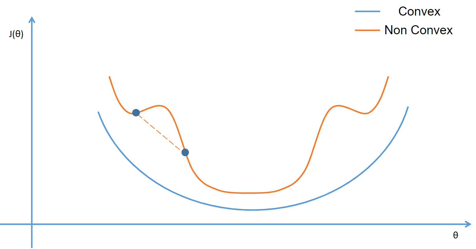
The cost function(\(J(\theta)\)) is a metric to measure how well the model/hypothesis($h_\theta(x)$) predicts outputs (Y) for a given input (X). The cost function used in Linear regression cannot be used here since it contains many minima since it is a non-convex function. The sigmoid function, which is our hypothesis, is non-linear and might get stuck in a local minima. Hence, we need a cost function that is convex in nature so that the gradient descent algorithm can reach the global minima.

So, to better understand this, let us consider that our hypothesis predicted a value $h_\theta(x) = 0.8$, which implies there is an 80% chance the patient is diabetic for given input parameters,

on the similar grounds, we can also state that there is an 20% of patient is not being diabetic,

Now, if the actual/correct value of Y = 1 for the given patient, from equation XX, we can conclude that our hypothesis has made a correct prediction as 1 since $h_\theta(x) = 0.8$, which is greater than 0.5. However, the problem arises when we try to calculate the error with the available cost function since it gives ‘0’ as an error.

here predicted output \(h_\theta(x)\) is diabetic(1) and actual output is also (Y = 1),

Hence, whenever there is a correct prediction, there is no scope for improvement with the current cost function, and with the same analogy for wrong prediction, the error will always be -1. To solve this problem, we devise a cost function with two components for each output.

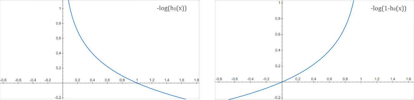
Whenever the actual/correct value of Y = 1, we expect the $h_\theta(x)$ to be 1 or close to 1. Hence, to measure the closeness towards the value 1, we use the function -log($h_\theta(x)$). The function will have the very least value when it is close to 1 and will become 0 when $h_\theta(x)$ becomes 1.

Whenever the actual/correct value of Y = 0, we expect the $h_\theta(x)$ to be 0 or very close to 0. Hence, to measure the closeness towards the value 0, we use the function -log(1 - $h_\theta(x)$). The function will have the very least value when it is close to 0 and will become 0 when $h_\theta(x)$ becomes 0.

so, we can formulate the cost function with both the components(functions) as,

We can further rewrite the cost function into one equation instead of having two separate functions for each output value.

4. Optimization

The cost function calculates the error for any given values of model parameters(\(\theta_0,\theta_1,\theta_2\ .\ .\theta_n\)), and the job of the optimization algorithm is to iteratively adjust the parameters based on the gradient (slope) of the cost function with respect to each parameter such that the error is minimized.

Hence, we initialize the model parameters with some initial values (hyperparameter initialization) that serve as the optimization process’s starting point and update them to minimize the error. With the initialized values for parameters, we will get an error value. Still, the challenge here is to decide with obtained error whether we should increase the value of parameters or decrease them so that the error will be reduced with the modified parameters. If we decide on the choice (increase/decrease), the next challenge is the magnitude with which we should update them. Hence we can roughly imagine this problem where the model parameters are like vector elements with scope for optimization in both magnitude and direction.

So, to minimize the error, with initial values for parameters, we calculate the gradient of the cost function with respect to each coefficient. The gradient descent is a first-order iterative optimization algorithm for finding a local minimum of a differentiable function. It calculates the partial derivative of the cost function(\(J\left(\theta\right)\)) with respect to each model parameter which represents the slope of the cost function in the direction of each parameter, indicating how the cost function changes with respect to changes in the parameters. After calculating gradients for each parameter, we update the parameter in the opposite direction by a small fraction (learning rate) since the gradient gives the direction of the steepest ascent. The learning rate is a hyperparameter that controls the step size taken in each iteration of the optimization process. It determines how large or small the coefficient updates should be to ensure the algorithm converges effectively without overshooting the minimum.

Hence, the generic parameter update formula is as follows, \(\theta∶=\theta\ – α \frac{\partial}{\partial\theta}J\left(\theta\right)\)

The gradients for all the parameters ($\theta_j$) should be calculated with respect to the current cost to update the the parameters,

\begin{equation} \theta_j∶=\theta_j\ – α \frac{\partial}{\partial\theta_j}J\left(\theta\right) \label{eq:1} \end{equation}

for all j = 0, 1, 2, 3, 4 , . . n

Let us simplify the update rule for each parameter by calculating the paritial derivate of the cost function(\(J(\theta)\)) with respect to each model parameter,

let us rewrite the cost function $J(\theta)$ for one sample for simplicity during the calculation of the partial derivate,

now we shall calculate the partial derivative of $J(\theta)$ with respect to each model parameter to identify how the error changes as you tweak each model parameter.

here \(h_{\theta}(x)\) is sigmoid function, where \(h_{\theta}(x)=\frac{1}{1+e^{-z}}\)

i. Derivative of sigmoid function:

before processding further, let us calculate the derivative sigmoid function first as it ease the work of calculating the partial derivative of cost function $J(\theta)$ with respect to each model parameter

take the derivative using the quotient rule like, if Let f(x)=g(x)/h(x), then according quotient rule

We have calculated the derivative but we still need to simplify it to get into the form which is very useful in Machine Learning specifically in neural networks to backpropagate through sigmoid activation functions. To simplify let us add and subtract the value 1 in the numerator.

Now we can rewrite the fraction by breaking into two terms.

If we closely observe both the terms have sigmoid component and we can take that outside

since $h_{\theta}(x)=\frac{1}{1+e^{-z}}$ we can replace $\frac{1}{1+e^{-z}}$ by $h_{\theta}(x)$ and the $\frac{d}{dx} h_{\theta}(x)$ will be as,

ii. Derivative of log loss cost function:

Now let us get back to original equation (XX) for calculating the paritial derivate of the cost function(\(J(\theta)\)) with respect to each model parameter,

since hypothesis $h_\theta(x) = g(z)$, where z = $\theta^{T} x$, we can replace $h_{\theta}(x)$ by $g(\theta^{T} x)$

by using the earlier calculated derivative of the sigmoid function, we can write the derivative of $g (\theta^{T} x)$ as $g(\theta^{T} x) (1-g(\theta^{T} x))$

the $\theta^{T}x$ = $\theta_{0} x_{0}+\theta_{1} x_{1}+\theta_{2} x_{2}+\ldots+\theta_{n} x_{n}$

we can replace $g (\theta^{T} x)$ by $h_{\theta}(x)$

let us substitute the value ($\left(h_\theta\left(x\right)-y\right).x_j$) obtained by calculating paritial derivate of the cost function into the original parameter update equation \eqref{eq:1},

using the update rule, we should update all model parameters ($\theta_j$) to minimize the cost/error at every iteration(epoch), so that error reaches a mimima.

.. .. .. ..

.. .. .. ..

The parameter optimization process is performed in an iterative loop (epoch) until model parameters converge, since the gradient will be theoretically zero at that point(slope will be zero), where the cost function reaches a minimum value.

The Hyperparameter Epochs define the number of times we perform the optimization process. As we progress with the optimization process with a predefined number of epochs, the error from the model starts decreasing. As said earlier, Gradient descent is one such iterative optimization algorithm used to learn the Linear Regression model parameters to minimize the cost/error. The gradient descent algorithm has three variations based on the number of samples(m) considered for calculating the error and optimizing the model parameters for convergence.

Since the training data is exposed to the model during the training(parameter optimization) process, we use the testing data to verify how the model performs on unseen data after every epoch.

The learning algorithm will be initialized with a predefined number of epochs and learning rate. Depending on the number of features, corresponding number of parameters are created, and all are initialized with value zero.

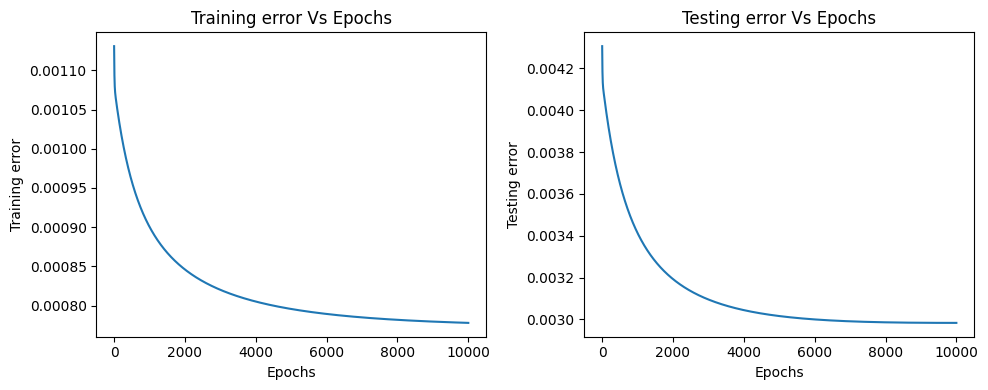
The following section shows the training progress with the intermediate, final training, and testing errors. It also shows the parameter values at respective epochs during the training.

Epoch: 1000 Training error: 0.0009004805124261176 Testing error: 0.0034131232876424577 Train accuarcy: 73.89162561576354 Testing accuarcy: 71.25 Parameters: [-2.329310329301874, 0.9227513039462504, 1.8920983939691118, -0.7547894465461735, 0.10754102528301454, 0.5488721666222018, 0.8146392056989059, 0.774618694550216, 0.8975613043084261]
Epoch: 2000 Training error: 0.000845976807802336 Testing error: 0.0031930841399454833 Train accuarcy: 75.53366174055829 Testing accuarcy: 78.125 Parameters: [-3.541716842093086, 1.2277918206917384, 3.082934863983692, -1.0279199084231998, 0.15530392643265076, 0.6405021542851494, 1.6450799730737198, 1.2101147188306078, 1.0252254042310465]
Epoch: 3000 Training error: 0.0008200171825445853 Testing error: 0.003095493287354257 Train accuarcy: 76.35467980295566 Testing accuarcy: 78.125 Parameters: [-4.3764575127515455, 1.3902258954355058, 3.8575132464676893, -1.1556586181432267, 0.14013558789524838, 0.5558068056879106, 2.344707020091758, 1.4735136574075625, 0.9879657804819949]
Epoch: 4000 Training error: 0.0008050511115281338 Testing error: 0.0030446887755775543 Train accuarcy: 77.66830870279146 Testing accuarcy: 78.125 Parameters: [-5.001597879266854, 1.5054201285353548, 4.395981655246799, -1.215061832134734, 0.10424958524392225, 0.41321294787947005, 2.9342022945068407, 1.6529521488287668, 0.9184931226941946]
Epoch: 5000 Training error: 0.0007955633563012411 Testing error: 0.003016359268316165 Train accuarcy: 77.83251231527095 Testing accuarcy: 77.5 Parameters: [-5.492309533745572, 1.5960874499539834, 4.788125745696554, -1.2412839055800502, 0.06535045148474555, 0.2603808774070449, 3.4342431355801732, 1.786196874801087, 0.8496056950181817]
Epoch: 6000 Training error: 0.0007892161220036542 Testing error: 0.003000227122445876 Train accuarcy: 77.504105090312 Testing accuarcy: 78.125 Parameters: [-5.888940295435089, 1.6700041388539368, 5.084007349433413, -1.2514736323573794, 0.029546739272138866, 0.11641403068958778, 3.861238485557505, 1.8909307127704105, 0.7897970496498945]
Epoch: 7000 Training error: 0.0007848230009684198 Testing error: 0.0029911761126428654 Train accuarcy: 77.66830870279146 Testing accuarcy: 78.75 Parameters: [-6.215891544391767, 1.7310758880011419, 5.313580212539376, -1.2542263336185537, -0.0016907411218878318, -0.011878538780032475, 4.22798276226333, 1.9762528763350027, 0.7404292898643329]
Epoch: 8000 Training error: 0.0007817097792924103 Testing error: 0.00298639335982755 Train accuarcy: 77.83251231527095 Testing accuarcy: 78.75 Parameters: [-6.489186365317914, 1.7818778535069846, 5.495712275578323, -1.2538564054829628, -0.028552649372366012, -0.12308358066100278, 4.544557605354781, 2.047314834837199, 0.70062746406079]
Epoch: 9000 Training error: 0.0007794643941099702 Testing error: 0.002984234031815644 Train accuarcy: 77.99671592775042 Testing accuarcy: 78.75 Parameters: [-6.719994428343702, 1.8243440643771562, 5.642795559028178, -1.2524816624817257, -0.051702253488385204, -0.21808185082114703, 4.819010557103963, 2.1073186964750854, 0.6689107625448427]
Epoch: 10000 Training error: 0.0007778224069240032 Testing error: 0.0029836971903924076 Train accuarcy: 77.99671592775042 Testing accuarcy: 78.75 Parameters: [-6.9164602903251104, 1.8599998964138647, 5.763269718689498, -1.2510853936596698, -0.071834409080901, -0.2986163748632091, 5.057840147992185, 2.158431004065721, 0.6437756831501521]



-----------------------------------------------------Training Finished-----------------------------------------------------

Best test accuaracy: 78.75 is at epoch: 1784 with train accuarcy: 75.86206896551724 test_error: 0.003225498224363808 and with parameters [-3.320876767133666, 1.1805319398626033, 2.8700767098557454, -0.9852342639982549, 0.15240185791118044, 0.6420294034836616, 1.4772869530312023, 1.1352877811767579, 1.0204168092136399]

---------------------------------------------------------------------------------------------------------------------------

Graph plots to visualize how the training and testing errors are decresing as the model starts training.

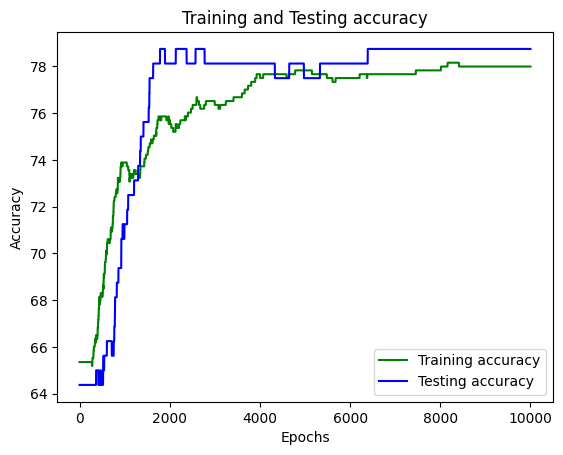
Graph plots to visualize how the training and testing accuracy are increasing as the model starts training.

5. Logistic Regresion with Scikit library

Now, let us use the scikit-learn machine learning library to implement the Logistic Regression algorithm and analyze the results.

The testing accuracy of the model is 78.125
The training accuracy of the model is 77.33990147783251

We can observe here that the error from the scikit testing accuracy of the model is $78.125$ and training accuracy of the model is $77.33990147783251$. from our implementation, we obtained Best test accuaracy: $78.75$ and train accuarcy: $75.86206896551724$. Here, we can tell that testing accurcay from our implementation is less than the scikit library implementation.

Now, let us also cross-check whether our accurcay calculation function has correctly predicted the accuracy by substituting the optimized model parameters from our implementation into the scikit model and calculating the accuracy.

The testing accuracy of the model is 78.75
The training accuracy of the model is 75.86206896551724

6. Complete code Logistic Regression

7. References:

1. Machine Learning, Tom Mitchell, McGraw Hill, 1997.
2. “CS229: Machine Learning” course by Andrew N G at Stanford, Autumn 2018.