This post provides an in-depth discussion of the Linear Regression algorithm and its implementation from scratch using Python.

Introduction

Linear Regression is a Supervised Learning algorithm used to solve problems where for every input(X), the respective output (Y) values are always continuous, and the Logistic Regression algorithm is employed when output (Y) values are discrete. Linear Regression aims to find the best-fitting straight line (a linear equation) representing the relationship between the inputs and the target variable. Now, to understand the Linear Regression algorithm, let us look into some real-world problems that can be solved with this algorithm’s help.

• Number of customers visiting the shop –> Profit for the shop owner
• Size of pizza –> Price of pizza
• Years of experience –> Salary of an employee
• Area of the house –> Price of the house

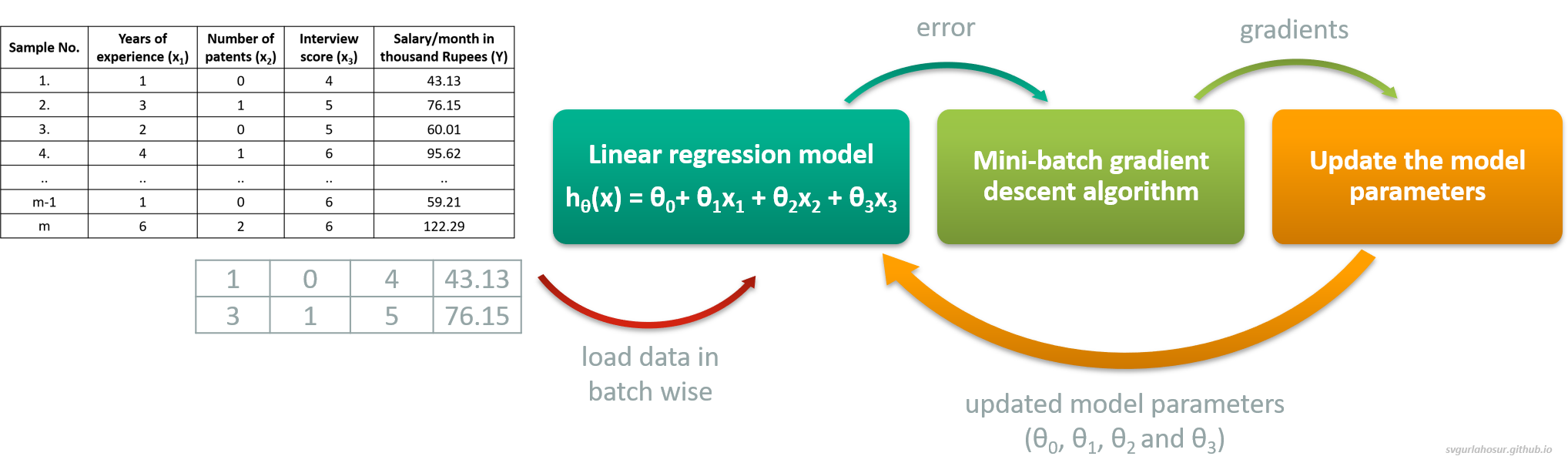
In all these examples, output/predicted values are continuous; hence, Linear Regression is used to build the machine learning model (hypothesis) and predict the output for a new set of inputs. To understand the working of the Linear Regression algorithm from a practical perspective, let us consider the problem of predicting an employee’s salary based on various employee qualities. Now, to solve this problem to predict the employee salary with Linear Regression, we should apply the following four steps:

1. Data collection
2. Model/hypothesis representation
3. Cost calculation
4. Optimization of model parameters

1. Data Collection

Let us consider/collect sample data records of salary provided by the company to employees based upon one feature of employees, like years of experience. We call this Univariate Linear Regression since we use a single feature to predict the employee’s salary.

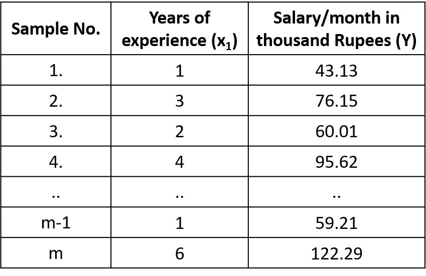
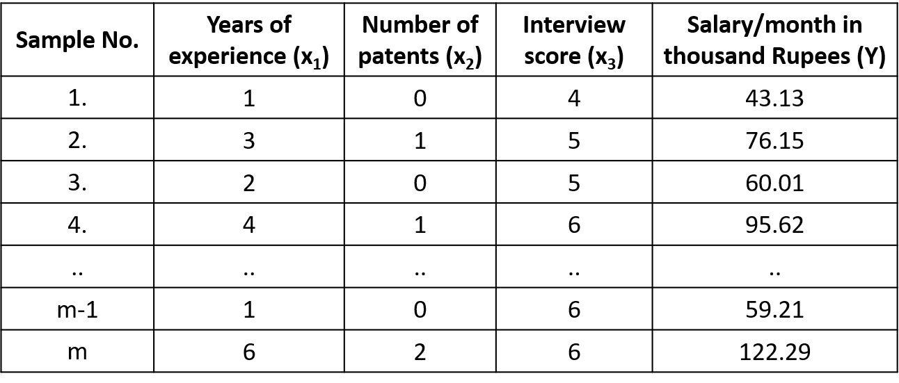
Instead of a single feature, if we use multiple features (qualities) of an employee to predict the salary, we call it Multi-variate Linear Regression.

Note:

1. Number of samples(records) range from 1, 2, 3, 4, . . . ., m.
2. Number of features range from $x_0, x_1, x_2, x_3, . . . . x_n$ where $x_0$ is considered as 1.
3. Notation used to identify the dataset(superscript indicates the sample number and subscript indicates the feature number): $x^2$ - (3, 1, 5), $x^2_1$ - 3, $x^2_2$ - 1 and $x^4$ - (4, 1, 6).

Visit the training and testing for the complete data.

2. Model/hypothesis represenation

The model/hypothesis ($h_\theta(x)$) approximates the target function by finding the relationship (pattern) between input features and output using linear operators (since data is linear). Hence we can define the hypothesis for Linear Regression algorithm as,

and we can rewrite the hypothesis $h_\theta(x)$ as, $h_\theta\left(x\right)=\sum_{j=0}^{n}{\theta_jx_j}$

where $_\ \theta_0,\ \theta_1,\ \theta_2,\ \theta_3,\ \theta_4,\ .\ .\ \theta_n$ are model parameters and $x_0, x_1, x_2, x_3, x_4,\ .\ .\ .x_n$ are input features($x_0$ = 1).

3. Cost function

The cost function ($J(\theta)$) is a metric to measure how well the model/hypothesis ($h_\theta(x)$) predicts outputs (Y) for a given input (X). It calculates the average squared difference (MSE) between the predicted output from the model/hypothesis and actual output values. By convention, we put a one-half ($1/2$) constant to average squared difference (MSE) because, when we take the derivative of the cost function with respect to each model parameter for minimizing error, it will make some of the math a little bit simpler. The Linear Regression algorithm aims to minimize the cost(error) by finding the optimized values for model parameters.

where m = number of samples/records considered for calculating the cost/error

An optimization algorithm is used to iteratively update the model parameters until convergence, where the cost function reaches a minimum value. Gradient descent is one such iterative optimization algorithm used to learn the Linear Regression model parameters to minimize the cost/error.

4. Optimization of model parameters

The cost function calculates the error for any given values of model parameters (\(\theta_0,\theta_1,\theta_2\ .\ .\theta_n\)), and the job of the optimization algorithm is to iteratively adjust the parameters based on the gradient (slope) of the cost function with respect to each parameter such that the error is minimized.

Hence, we initialize the model parameters with some initial values (hyperparameter initialization) that serve as the optimization process’s starting point and update them to minimize the error. With the initialized values for parameters, we will get an error value. Still, the challenge here is to decide with obtained error whether we should increase the value of parameters or decrease them so that the error will be reduced with the modified parameters. If we decide on the choice (increase/decrease), the next challenge is the magnitude with which we should update them. Hence we can roughly imagine this problem where the model parameters are like vector elements with scope for optimization in both magnitude and direction.

So, to minimize the error, with initial values for parameters, we calculate the gradient of the cost function with respect to each coefficient. The gradient descent is a first-order iterative optimization algorithm for finding a local minimum of a differentiable function. It calculates the partial derivative of the cost function (\(J\left(\theta\right)\)) with respect to each model parameter which represents the slope of the cost function in the direction of each parameter, indicating how the cost function changes with respect to changes in the parameters. After calculating gradients for each parameter, we update the parameter in the opposite direction by a small fraction (learning rate) since the gradient gives the direction of the steepest ascent. The learning rate is a hyperparameter that controls the step size taken in each iteration of the optimization process. It determines how large or small the coefficient updates should be to ensure the algorithm converges effectively without overshooting the minimum.

Hence, the generic parameter update formula is as follows, \(\theta∶=\theta\ – α \frac{\partial}{\partial\theta}J\left(\theta\right)\)

The gradients for all the parameters ($\theta_j$) should be calculated with respect to the current cost to update the the parameters,

\begin{equation} \theta_j∶=\theta_j\ – α \frac{\partial}{\partial\theta_j}J\left(\theta\right) \label{eq:1} \end{equation}

for all j = 0, 1, 2, 3, 4 , . . n

Let us simplify the update rule for each parameter in the equation \eqref{eq:1} by calculating the paritial derivate of the cost function ($\frac{\partial}{\partial\theta_j}J\left(\theta\right)$) with respect to each model parameter,

let us substitute the value ($\left(h_\theta\left(x\right)-y\right).x_j$) obtained by calculating paritial derivate of the cost function into the original parameter update equation \eqref{eq:1},

using the update rule, we should update all model parameters ($\theta_j$) to minimize the cost/error at every iteration(epoch), so that error reaches a mimima.

.. .. .. ..

.. .. .. ..

The parameter optimization process is performed in an iterative loop (epoch) until model parameters converge, since the gradient will be theoretically zero at that point(slope will be zero), where the cost function reaches a minimum value.

The Hyperparameter Epochs define the number of times we perform the optimization process. As we progress with the optimization process with a predefined number of epochs, the error from the model starts decreasing. As said earlier, Gradient descent is one such iterative optimization algorithm used to learn the Linear Regression model parameters to minimize the cost/error. The gradient descent algorithm has three variations based on the number of samples(m) considered for calculating the error and optimizing the model parameters for convergence.

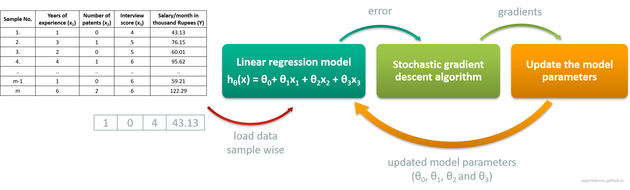
i. Stochastic gradient descent:

A single sample is used at every iteration to predict model output, calculate the error, and optimize the model parameters. This method is straightforward but computationally expensive to train models on large datasets with all samples. It can quickly give an insight into the model performance and converge faster, making it ideal for large datasets. The frequent updates can help escape local minima, but the noisy updates sometimes may lead to erratic convergence.

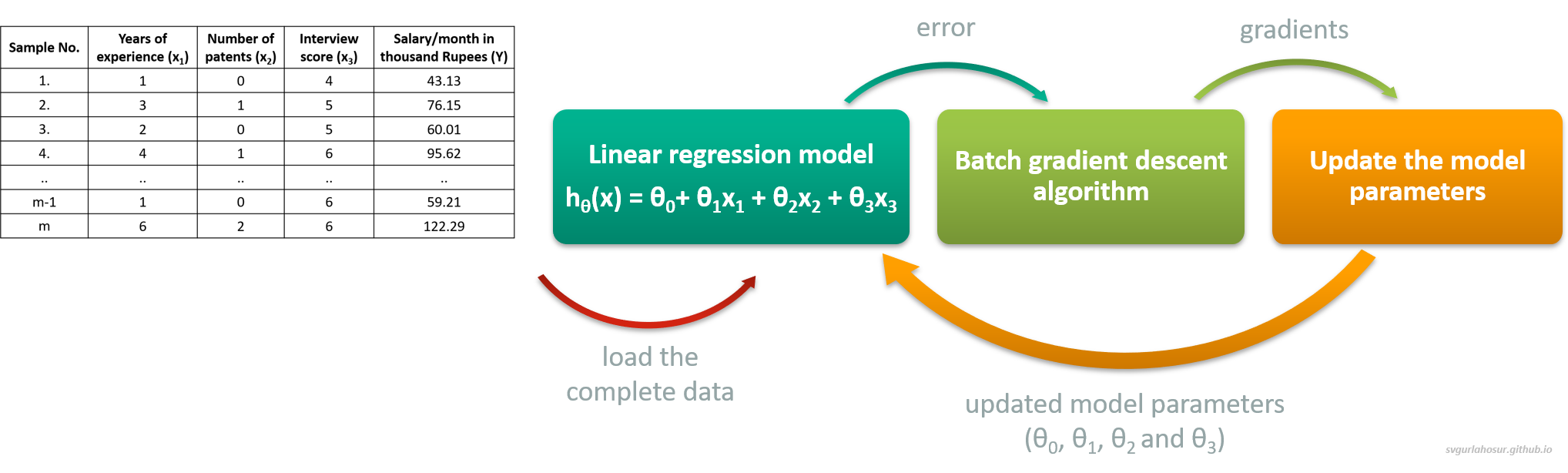
ii. Batch gradient descent:

All the samples are used at every iteration to predict model output and calculate the error, resulting in a more accurate and stable estimation of gradients to optimize the model parameters. This method is ideal for convex or well-behaved loss surfaces, guaranteeing convergence to the global minimum. At the same time, this method is computationally expensive since the entire training dataset is loaded onto memory, particularly for larger datasets. This method will also struggle with non-convex loss surfaces and sometimes may lead to early convergence (local minima) with a less optimized set of parameters.

iii. Mini batch gradient:

A batch of samples is used at every iteration to predict model output, calculate the error, and optimize the model parameters. This method combines the advantages of stochastic gradient descent and batch gradient descent by processing a random subset (mini-batch) of the samples at each iteration, making the model both stable and efficient. This method offers parallelism opportunities and can take advantage of hardware acceleration, and it is the most commonly used optimization of Deep Learning algorithms due to its scalability and versatility. Careful tuning of the batch size and learning rate can be used to balance computational efficiency and parameter update stability. Otherwise, it can lead to suboptimal convergence or inefficient models.

Note: All the code snippets are based on the Stochastic gradient descent algorithm and refer the Batch gradient descent and Mini batch gradient for respective implementaion.

Since the training data is exposed to the model during the training(parameter optimization) process, we use the testing data to verify how the model performs on unseen data after every epoch.

The learning algorithm will be initialized with a predefined number of epochs and learning rate. Depending on the number of features, corresponding number of parameters are created, and all are initialized with value zero.

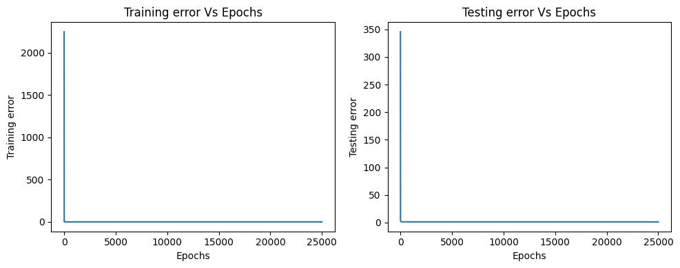
The following section shows the training progress with the intermediate, final training, and testing errors. It also shows the parameter values at respective epochs during the training.

Epoch: 2000 Training error: 0.6751715413266479 Testing_error: 1.183341917528965 Parameters: [-0.255538575759327, 9.485931764649, 6.078472111746896, 8.47518648378849]
Epoch: 4000 Training error: 0.6742278755388742 Testing_error: 1.1764871600965758 Parameters: [-0.38363349332072405, 9.489784692176048, 6.0786361313358785, 8.489563304720935]
Epoch: 6000 Training error: 0.6742003164773049 Testing_error: 1.175968080596902 Parameters: [-0.3936962887428751, 9.490087367896683, 6.078649016277748, 8.490692709467186]
Epoch: 8000 Training error: 0.6741984389235399 Testing_error: 1.1759274228907803 Parameters: [-0.3944867951394988, 9.490111145294827, 6.07865002848446, 8.490781432494813]
Epoch: 10000 Training error: 0.6741982932016067 Testing_error: 1.1759242296689814 Parameters: [-0.39454889521573566, 9.490113013183876, 6.0786501080007165, 8.490788402339469]
Epoch: 12000 Training error: 0.6741982817650337 Testing_error: 1.1759239788225648 Parameters: [-0.39455377363228045, 9.490113159920252, 6.078650114247313, 8.490788949871897]
Epoch: 14000 Training error: 0.6741982808666698 Testing_error: 1.1759239591167399 Parameters: [-0.3945541568676921, 9.490113171447494, 6.078650114738017, 8.490788992884577]
Epoch: 16000 Training error: 0.6741982807960991 Testing_error: 1.1759239575687033 Parameters: [-0.3945541869736474, 9.49011317235303, 6.078650114776581, 8.490788996263545]
Epoch: 18000 Training error: 0.6741982807905543 Testing_error: 1.1759239574471043 Parameters: [-0.3945541893386998, 9.490113172424172, 6.07865011477959, 8.490788996528988]
Epoch: 20000 Training error: 0.6741982807901219 Testing_error: 1.1759239574375986 Parameters: [-0.39455418952452476, 9.490113172429727, 6.078650114779848, 8.49078899654986]
Epoch: 22000 Training error: 0.6741982807900848 Testing_error: 1.1759239574367917 Parameters: [-0.39455418953910915, 9.490113172430192, 6.078650114779855, 8.490788996551487]
Epoch: 24000 Training error: 0.6741982807900817 Testing_error: 1.1759239574367288 Parameters: [-0.3945541895403048, 9.490113172430219, 6.0786501147799274, 8.490788996551608]



-----------------------------------------------------Training Finished-----------------------------------------------------

The Best testing error: 1.1759239574367126 is at epoch: 23606 with parameters values [-0.3945541895403048, 9.490113172430219, 6.0786501147799274, 8.490788996551608]

---------------------------------------------------------------------------------------------------------------------------

Graph plots to visualize how the training and testing errors are decresing as the model starts training.

5. Linear Regresion with Scikit library

Now, let us use the scikit-learn machine learning library to implement the Linear Regression algorithm and analyze the results.

The testing error is: 1.2169218827800505 with intercept: -0.4080644275995269 and coefficients: [9.49049716 6.06819016 8.48657175]

We can observe here that the error from the scikit is $1.2169218827800505$, and from our stochastic gradient descent algorithm, we obtained an error of $1.1759239574367126$. Here, we can tell the error from the stochastic gradient descent algorithm is less than the scikit library implementation. Still, the dataset we have considered is a non-standard dataset, and when we consider the real-time or standard datasets, the results may vary.

Note:

1. If you are still thinking about why the mean squared error(mse) value is divided by 2, please refer to the Stanford CS229: Machine Learning - Linear Regression and Gradient Descent from Andrew N G.

We should also observe that the dataset is not normalized when implementing Stochastic Gradient Descent Linear Regression. When trying to apply this code over any standard dataset, normalize the dataset so that all features in the dataset to a common scale without distorting differences in the ranges of values and stable model performance during machine learning.

Now, let us also cross-check whether our cost calculation function has correctly predicted the error by substituting the optimized model parameters from our stochastic gradient descent algorithm into the scikit model and calculating the test error.

The testing error is: 1.1759239574367335 with intercept: -0.3945541895403048 and coefficients: [9.49011317 6.07865011 8.490789  ]

6. Complete code with Stochastic Gradient Descent

The complete code for Linear Regression with stochastic gradient descent algorithm is as follows.

7. References:

1. Machine Learning, Tom Mitchell, McGraw Hill, 1997.
2. “CS229: Machine Learning” course by Andrew N G at Stanford, Autumn 2018.